|
|
| Line 1: |
Line 1: |
| {{More footnotes|date=June 2009}}
| | In [[computer science]], the '''Edmonds–Karp algorithm''' is an implementation of the [[Ford–Fulkerson algorithm|Ford–Fulkerson method]] for computing the [[maximum flow problem|maximum flow]] in a [[flow network]] in ''[[big O notation|O]]''(''V'' ''E''<sup>2</sup>) time. The algorithm was first published by Yefim (Chaim) Dinic in 1970<ref>{{cite journal |first=E. A. |last=Dinic |title=Algorithm for solution of a problem of maximum flow in a network with power estimation |journal=Soviet Math. Doklady |volume=11 |issue= |pages=1277–1280 |publisher=Doklady |year=1970 |url= |doi= |id= |accessdate= }}</ref> and independently published by [[Jack Edmonds]] and [[Richard Karp]] in 1972.<ref>{{cite journal |last1=Edmonds |first1=Jack |author1-link=Jack Edmonds |last2=Karp |first2=Richard M. |author2-link=Richard Karp |title=Theoretical improvements in algorithmic efficiency for network flow problems |journal=Journal of the ACM |volume=19 |issue=2 |pages=248–264 |publisher=[[Association for Computing Machinery]] |year=1972 |url= |doi=10.1145/321694.321699 |id= |accessdate= }}</ref> [[Dinic's algorithm]] includes additional techniques that reduce the running time to ''O''(''V''<sup>2</sup>''E''). |
| [[Image:Random Walk example.svg|thumb|right|420px|Example of eight random walks in one dimension starting at 0. The plot shows the current position on the line (vertical axis) versus the time steps (horizontal axis).]] | |
| A '''random walk''' is a [[mathematical]] formalization of a path that consists of a succession of [[random]] steps. For example, the path traced by a [[molecule]] as it travels in a liquid or a gas, the search path of a [[foraging]] animal, the price of a fluctuating [[random walk hypothesis|stock]] and the financial status of a [[gambler]] can all be ''modeled'' as random walks, although they may not be truly random in reality. The term ''random walk'' was first introduced by [[Karl Pearson]] in 1905.<ref>Pearson, K. (1905). ''The Problem of the Random Walk.'' [[Nature (journal)|Nature]]. '''72''', 294.</ref> Random walks have been used in many fields: [[ecology]], [[economics]], [[psychology]], [[computer science]], [[physics]], [[chemistry]], and [[biology]].<ref name=[1]>Van Kampen N. G., Stochastic Processes in Physics and Chemistry, revised and enlarged edition (North-Holland, Amsterdam) 1992.</ref><ref name=[2]>Redner S., A Guide to First-Passage Process (Cambridge University Press, Cambridge, UK) 2001.</ref><ref name=[3]>Goel N. W. and Richter-Dyn N., Stochastic Models in Biology (Academic Press, New York) 1974.</ref><ref name=[4]>Doi M. and Edwards S. F., The Theory of Polymer Dynamics (Clarendon Press, Oxford) 1986</ref><ref name=[4c]>De Gennes P. G., Scaling Concepts in Polymer Physics (Cornell University Press, Ithaca and London) 1979.</ref><ref name=[5]>Risken H., The Fokker–Planck Equation (Springer, Berlin) 1984.</ref><ref name=[6]>Weiss G. H., Aspects and Applications of the Random Walk (North-Holland, Amsterdam) 1994.</ref><ref name=[7]>Cox D. R., Renewal Theory (Methuen, London) 1962.</ref> Random walks explain the observed behaviors of processes in these fields, and thus serve as a fundamental [[Statistical model|model]] for the recorded [[Stochastic process|stochastic activity]].
| |
|
| |
|
| Various different types of random walks are of interest. Often, random walks are assumed to be [[Markov chain]]s or [[Markov process]]es, but other, more complicated walks are also of interest. Some random walks are on [[graph theory|graphs]], others on the line, in the plane, or in higher dimensions, while some random walks are on [[group theory|groups]]. Random walks also vary with regard to the time parameter. Often, the walk is in discrete time, and indexed by the natural numbers, as in <math>X_0,X_1,X_2,\dots</math>. However, some walks take their steps at random times, and in that case the position <math>X_t</math> is defined for the continuum of times <math>t\ge 0</math>. Specific cases or limits of random walks include the [[Lévy flight]]. Random walks are related to the [[diffusion]] models and are a fundamental topic in discussions of [[Markov process]]es. Several properties of random walks, including dispersal distributions, first-passage times and encounter rates, have been extensively studied.
| | ==Algorithm== |
|
| |
|
| ==Lattice random walk==
| | The algorithm is identical to the [[Ford–Fulkerson algorithm]], except that the search order when finding the [[augmenting path]] is defined. The path found must be a shortest path that has available capacity. This can be found by a [[breadth-first search]], as we let edges have unit length. The running time of ''O''(''V'' ''E''<sup>2</sup>) is found by showing that each augmenting path can be found in ''O''(''E'') time, that every time at least one of the ''E'' edges becomes saturated (an edge which has the maximum possible flow), that the distance from the saturated edge to the source along the augmenting path must be longer than last time it was saturated, and that the length is at most ''V''. Another property of this algorithm is that the length of the shortest augmenting path increases monotonically. There is an accessible proof in ''[[Introduction to Algorithms]]''.<ref>{{cite book |author=[[Thomas H. Cormen]], [[Charles E. Leiserson]], [[Ronald L. Rivest]] and [[Clifford Stein]] |title=[[Introduction to Algorithms]] |publisher=MIT Press | year = 2009 |isbn=978-0-262-03384-8 |edition=third |chapter=26.2 |pages=727–730 }}</ref> |
| {{Refimprove section|date=April 2011|reason=no sources in this entire section}}
| |
| A popular random walk model is that of a random walk on a regular lattice, where at each step the location jumps to another site according to some probability distribution. In a '''simple random walk''', the location can only jump to neighboring sites of the lattice. In ''' simple symmetric random walk''' on a locally finite lattice, the probabilities of the location jumping to each one of its immediate neighbours are the same. The best studied example is of random walk on the ''d''-dimensional integer lattice (sometimes called the hypercubic lattice) <math>\mathbb Z^d</math>.<ref>Révész Pal, Random walk in random and non random environments, World Scientific, 1990</ref>
| |
|
| |
|
| ===One-dimensional random walk=== | | ==Pseudocode== |
| An elementary example of a random walk is the random walk on the [[integer]] number line, <math>\mathbb Z</math>, which starts at 0 and at each step moves +1 or −1 with equal probability.
| | {{Wikibooks|Algorithm implementation|Graphs/Maximum flow/Edmonds-Karp|Edmonds-Karp}} |
|
| |
|
| This walk can be illustrated as follows. A marker is placed at zero on the number line and a fair coin is flipped. If it lands on heads, the marker is moved one unit to the right. If it lands on tails, the marker is moved one unit to the left. After five flips, the marker could now be on 1, −1, 3, −3, 5, or −5. With five flips, three heads and two tails, in any order, will land on 1. There are 10 ways of landing on 1 (by flipping three heads and two tails), 10 ways of landing on −1 (by flipping three tails and two heads), 5 ways of landing on 3 (by flipping four heads and one tail), 5 ways of landing on −3 (by flipping four tails and one head), 1 way of landing on 5 (by flipping five heads), and 1 way of landing on −5 (by flipping five tails). See the figure below for an illustration of the possible outcomes of 5 flips.
| | :''For a more high level description, see [[Ford–Fulkerson algorithm]]. |
|
| |
|
| [[Image:Flips.svg|thumb|800px|center|All possible random walk outcomes after 5 flips of a fair coin]] | | '''algorithm''' EdmondsKarp |
| [[Image:random walk 2500.svg|right|thumb|280px|Random walk in two dimensions ([http://upload.wikimedia.org/wikipedia/commons/f/f3/Random_walk_2500_animated.svg animated version])]] | | '''input''': |
| [[Image:random walk 25000 not animated.svg|right|thumb|280px|Random walk in two dimensions with 25 thousand steps ([http://upload.wikimedia.org/wikipedia/commons/c/cb/Random_walk_25000.svg animated version])]]
| | C[1..n, 1..n] ''(Capacity matrix)'' |
| [[Image:Random walk 2000000.png|right|thumb|280px|Random walk in two dimensions with two million even smaller steps. This image was generated in such a way that points that are more frequently traversed are darker. In the limit, for very small steps, one obtains [[Brownian motion]].]]
| | E[1..n, 1..?] ''(Neighbour lists)'' |
| | s ''(Source)'' |
| | t ''(Sink)'' |
| | '''output''': |
| | f ''(Value of maximum flow)'' |
| | F ''(A matrix giving a legal flow with the maximum value)'' |
| | f := 0 ''(Initial flow is zero)'' |
| | F := '''array'''(1..n, 1..n) ''(Residual capacity from u to v is C[u,v] - F[u,v])'' |
| | '''forever''' |
| | m, P := BreadthFirstSearch(C, E, s, t, F) |
| | '''if''' m = 0 |
| | '''break''' |
| | f := f + m |
| | ''(Backtrack search, and write flow)'' |
| | v := t |
| | '''while''' v ≠ s |
| | u := P[v] |
| | F[u,v] := F[u,v] + m |
| | F[v,u] := F[v,u] - m |
| | v := u |
| | '''return''' (f, F) |
|
| |
|
| To define this walk formally, take independent random variables <math>Z_1, Z_2,\dots</math>, where each variable is either 1 or −1, with a 50% probability for either value, and set <math>S_0 = 0\,\!</math> and <math>S_n =\sum_{j=1}^nZ_j.</math> The [[Series (mathematics)|series]] <math>\{S_n\}\,\!</math> is called the '''simple random walk on <math>\mathbb Z</math>'''. This series (the sum of the sequence of −1s and 1s) gives the distance walked, if each part of the walk is of length one.
| | '''algorithm''' BreadthFirstSearch |
| The [[expected value|expectation]] <math>E(S_n)\,\!</math> of <math>S_n\,\!</math> is zero. That is, the mean of all coin flips approaches zero as the number of flips increases. This follows by the finite additivity property of expectation:
| | '''input''': |
| | C, E, s, t, F |
| | '''output''': |
| | M[t] ''(Capacity of path found)'' |
| | P ''(Parent table)'' |
| | P := '''array'''(1..n) |
| | '''for''' u '''in''' 1..n |
| | P[u] := -1 |
| | P[s] := -2 ''(make sure source is not rediscovered)'' |
| | M := '''array'''(1..n) ''(Capacity of found path to node)'' |
| | M[s] := ∞ |
| | Q := queue() |
| | Q.offer(s) |
| | '''while''' Q.size() > 0 |
| | u := Q.poll() |
| | '''for''' v '''in''' E[u] |
| | ''(If there is available capacity, and v is not seen before in search)'' |
| | '''if''' C[u,v] - F[u,v] > 0 '''and''' P[v] = -1 |
| | P[v] := u |
| | M[v] := min(M[u], C[u,v] - F[u,v]) |
| | '''if''' v ≠ t |
| | Q.offer(v) |
| | '''else''' |
| | '''return''' M[t], P |
| | '''return''' 0, P |
|
| |
|
| :<math>E(S_n)=\sum_{j=1}^n E(Z_j)=0.</math>
| |
|
| |
|
| A similar calculation, using the independence of the random variables and the fact that <math>E(Z_n^2)=1</math>, shows that:
| | :''EdmondsKarp pseudo code using Adjacency nodes. |
|
| |
|
| :<math>E(S_n^2)=\sum_{j=1}^n E(Z_j^2)+ \sum_{i=1}^n \sum_{j=1}^n 2E(Z_j Z_i)=n.</math> | | '''algorithm''' EdmondsKarp |
| | '''input''': |
| | graph ''(Graph with list of Adjacency nodes with capacities,flow,reverse and destinations)'' |
| | s ''(Source)'' |
| | t ''(Sink)'' |
| | '''output''': |
| | flow ''(Value of maximum flow)'' |
| | flow := 0 ''(Initial flow to zero)'' |
| | q := '''array'''(1..n) ''(Initialize q to graph length)'' |
| | '''while''' true |
| | qt := 0 ''(Variable to iterate over all the corresponding edges for a source)'' |
| | q[qt+1] := s ''(initialize source array)'' |
| | pred := '''array'''(q.length) ''(Initialize predecessor List with the graph length)'' |
| | '''for''' qh=0;qh < qt && pred[t] := null |
| | cur := q[qh] |
| | for (graph[cur]) ''(Iterate over list of Edges)'' |
| | Edge[] e := graph[cur] ''(Each edge should be associated with Capacity)'' |
| | if pred[e.t] == null && e.cap > e.f |
| | pred[e.t] := e |
| | q[qt++] : = e.t |
| | if pred[t] = null |
| | break |
| | int df := MAX VALUE ''(Initialize to max integer value)'' |
| | for u = t; u != s; u = pred[u].s |
| | df := min(df, pred[u].cap - pred[u].f) |
| | for u = t; u != s; u = pred[u].s |
| | pred[u].f := pred[u].f + df |
| | pEdge := '''array'''(PredEdge) |
| | pEdge := graph[pred[u].t] |
| | pEdge[pred[u].rev].f := pEdge[pred[u].rev].f - df; |
| | flow := flow + df |
| | '''return''' flow |
|
| |
|
| This hints that <math>E(|S_n|)\,\!</math>, the [[expected value|expected]] translation distance after ''n'' steps, should be [[Big O notation|of the order of]] <math>\sqrt n</math>. In fact,{{citation needed|date=April 2013}}
| | ==Example== |
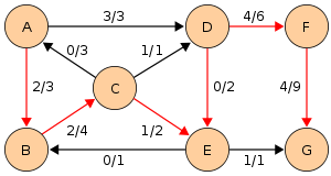
| | Given a network of seven nodes, source A, sink G, and capacities as shown below: |
|
| |
|
| :<math>\lim_{n\to\infty} \frac{E(|S_n|)}{\sqrt n}= \sqrt{\frac 2{\pi}}.</math> | | [[Image:Edmonds-Karp flow example 0.svg|300px]] |
|
| |
|
| This result shows that diffusion is ineffective for mixing because of the way the square root behaves for large <math>N</math>.{{citation needed|date=April 2013}}
| | In the pairs <math>f/c</math> written on the edges, <math>f</math> is the current flow, and <math>c</math> is the capacity. The residual capacity from <math>u</math> to <math>v</math> is <math>c_f(u,v)=c(u,v)-f(u,v)</math>, the total capacity, minus the flow that is already used. If the net flow from <math>u</math> to <math>v</math> is negative, it ''contributes'' to the residual capacity. |
|
| |
|
| How many times will a random walk cross a boundary line if permitted to continue walking forever? A simple random walk on <math>\mathbb Z</math> will cross every point an infinite number of times. This result has many names: the ''level-crossing phenomenon'', ''recurrence'' or the ''[[gambler's ruin]]''. The reason for the last name is as follows: a gambler with a finite amount of money will eventually lose when playing ''a fair game'' against a bank with an infinite amount of money. The gambler's money will perform a random walk, and it will reach zero at some point, and the game will be over.
| | {| class="wikitable" |
| | | |- |
| If ''a'' and ''b'' are positive integers, then the expected number of steps until a one-dimensional simple random walk starting at 0 first hits ''b'' or −''a'' is ''ab''. The probability that this walk will hit ''b'' before −''a'' is <math>a/(a+b)</math>, which can be derived from the fact that simple random walk is a [[martingale (probability theory)|martingale]].
| | !rowspan="2"| Capacity |
| <!-- Maybe a reference to the iterated log law should come here? -->
| | ! Path |
| | | |- |
| Some of the results mentioned above can be derived from properties of [[Pascal's triangle]]. The number of different walks of ''n'' steps where each step is +1 or −1 is 2<sup>''n''</sup>. For the simple random walk, each of these walks are equally likely. In order for ''S<sub>n</sub>'' to be equal to a number ''k'' it is necessary and sufficient that the number of +1 in the walk exceeds those of −1 by ''k''. The number of walks which satisfy <math>S_n=k</math> is equally the number of ways of choosing (''n'' + ''k'')/2 elements from an ''n'' element set,{{citation needed|date=September 2013}} denoted <math>n \choose (n+k)/2</math>. For this to be non-zero, it is necessary that ''n'' + ''k'' be an even number. Therefore, the probability that <math>S_n=k</math> is equal to <math>2^{-n}{n\choose (n+k)/2}</math>. By representing entries of Pascal's triangle in terms of [[factorial]]s and using [[Stirling formula|Stirling's formula]], one can obtain good estimates for these probabilities for large values of <math>n</math>.
| | ! Resulting network |
| | | |- |
| If the space is confined to <math>\mathbb Z</math>+ for brevity, the number of ways in which a random walk will land on any given number having five flips can be shown as {0,5,0,4,0,1}.
| | |rowspan="2"| <math>\min(c_f(A,D),c_f(D,E),c_f(E,G)) = </math><br> |
| | | <math>\min(3-0,2-0,1-0) = </math><br> |
| This relation with Pascal's triangle is demonstrated for small values of ''n''. At zero turns, the only possibility will be to remain at zero. However, at one turn, there is one chance of landing on −1 or one chance of landing on 1. At two turns, a marker at 1 could move to 2 or back to zero. A marker at −1, could move to −2 or back to zero. Therefore, there is one chance of landing on −2, two chances of landing on zero, and one chance of landing on 2.
| | <math>\min(3,2,1) = 1</math><br> |
| | | |align="center"| <math>A,D,E,G</math> |
| <!--[[Image:PascalTriangleRandomWalk.JPG|thumb|center|600px|Pascal's triangle in a random walk]] Commenting out previous table from pic--> | |
| {| class="wikitable" style="text-align:center"
| |
| |- | | |- |
| ! k
| | | [[Image:Edmonds-Karp flow example 1.svg|300px]]</td> |
| ! style="width:2em" | −5
| |
| ! style="width:2em" | −4
| |
| ! style="width:2em" | −3
| |
| ! style="width:2em" | −2
| |
| ! style="width:2em" | −1
| |
| ! style="width:2em" | 0
| |
| ! style="width:2em" | 1
| |
| ! style="width:2em" | 2
| |
| ! style="width:2em" | 3
| |
| ! style="width:2em" | 4
| |
| ! style="width:2em" | 5
| |
| |- | | |- |
| | <math>P[S_0=k]</math> | | |rowspan="2"| <math>\min(c_f(A,D),c_f(D,F),c_f(F,G)) = </math><br> |
| |
| | <math>\min(3-1,6-0,9-0) = </math><br> |
| |
| | <math>\min(2,6,9) = 2</math><br> |
| |
| | |align="center"| <math>A,D,F,G</math> |
| |
| |
| |
| |
| | 1
| |
| |
| |
| | | |
| |
| |
| |
| |
| | | |
| |- | | |- |
| | <math>2P[S_1=k]</math> | | | [[Image:Edmonds-Karp flow example 2.svg|300px]]</td> |
| |
| |
| |
| |
| |
| |
| |
| |
| | 1
| |
| |
| |
| | 1
| |
| |
| |
| |
| |
| |
| |
| |
| |
| |- | | |- |
| | <math>2^2P[S_2=k]</math> | | |rowspan="2"| <math>\min(c_f(A,B),c_f(B,C),c_f(C,D),c_f(D,F),c_f(F,G)) = </math><br> |
| |
| | <math>\min(3-0,4-0,1-0,6-2,9-2) = </math><br> |
| |
| | <math>\min(3,4,1,4,7) = 1</math><br> |
| |
| | |align="center"| <math>A,B,C,D,F,G</math> |
| | 1
| |
| |
| |
| | 2
| |
| |
| |
| | 1
| |
| | | |
| |
| |
| | | |
| |- | | |- |
| | <math>2^3P[S_3=k]</math> | | | [[Image:Edmonds-Karp flow example 3.svg|300px]]</td> |
| |
| |
| |
| |
| | 1
| |
| |
| |
| | 3
| |
| |
| |
| | 3
| |
| |
| |
| | 1
| |
| |
| |
| |
| |
| |- | | |- |
| | <math>2^4P[S_4=k]</math> | | |rowspan="2"| <math>\min(c_f(A,B),c_f(B,C),c_f(C,E),c_f(E,D),c_f(D,F),c_f(F,G)) = </math><br> |
| |
| | <math>\min(3-1,4-1,2-0,0-(-1),6-3,9-3) = </math><br> |
| | 1
| | <math>\min(2,3,2,1,3,6) = 1</math><br> |
| |
| | |align="center"| <math>A,B,C,E,D,F,G</math> |
| | 4
| |
| |
| |
| | 6
| |
| | | |
| | 4
| |
| |
| |
| | 1
| |
| | | |
| |- | | |- |
| | <math>2^5P[S_5=k]</math> | | | [[Image:Edmonds-Karp flow example 4.svg|300px]]</td> |
| | 1
| |
| |
| |
| | 5
| |
| |
| |
| | 10
| |
| |
| |
| | 10
| |
| |
| |
| | 5
| |
| |
| |
| | 1
| |
| |} | | |} |
|
| |
|
| The [[central limit theorem]] and the [[law of the iterated logarithm]] describe important aspects of the behavior of simple random walk on <math>\mathbb Z</math>. In particular, the former entails that as ''n'' increases, the probabilities (proportional to the numbers in each row) approach a [[normal distribution]].
| | Notice how the length of the [[augmenting path]] found by the algorithm (in red) never decreases. The paths found are the shortest possible. The flow found is equal to the capacity across the [[max flow min cut theorem|minimum cut]] in the graph separating the source and the sink. There is only one minimal cut in this graph, partitioning the nodes into the sets <math>\{A,B,C,E\}</math> and <math>\{D,F,G\}</math>, with the capacity |
| | | :<math>c(A,D)+c(C,D)+c(E,G)=3+1+1=5.\ </math> |
| As a direct generalization, one can consider random walks on crystal lattices (infinite-fold abelian covering graphs over finite graphs). Actually it is possible to establish the central limit theorem and large deviation theorem in this setting<ref>{{cite journal |author= M. Kotani, [[Toshikazu Sunada|T. Sunada]] |year= 2003 |title= Spectral geometry of crystal lattices |journal= Contemporary. Math.|volume= 338 |pages= 271–305 }}</ref>
| |
| .<ref>{{cite journal |author= M. Kotani, [[Toshikazu Sunada|T. Sunada]] |year= 2006 |title= Large deviation and the tangent cone at infinity of a crystal lattice |journal= Math. Z. |volume= 254 |pages= 837–870 }}</ref>
| |
| | |
| ====As a Markov chain====
| |
| A one-dimensional '''random walk''' can also be looked at as a [[Markov chain]] whose state space is given by the integers <math>i=0,\pm 1,\pm 2,\dots .</math> For some number ''p'' satisfying <math>\,0 < p < 1</math>, the transition probabilities (the probability ''P<sub>i,j</sub>'' of moving from state ''i'' to state ''j'') are given by
| |
| :<math>\,P_{i,i+1}=p=1-P_{i,i-1}.</math>
| |
| | |
| ===Higher dimensions===
| |
| [[Image:Walk3d 0.png|right|thumb|280px|Three random walks in three dimensions]]
| |
| Imagine now a drunkard walking randomly in an idealized city. The city is effectively infinite and arranged in a square grid, and at every intersection, the drunkard chooses one of the four possible routes (including the one he came from) with equal probability. Formally, this is a random walk on the set of all points in the [[Plane (mathematics)|plane]] with [[integer]] [[Coordinate system|coordinates]].
| |
| | |
| Will the drunkard ever get back to his home from the bar? This is the 2-dimensional equivalent of the level crossing problem discussed above. It turns out that he [[almost surely]] will in a 2-dimensional random walk, but for 3 dimensions or higher, the probability of returning to the origin decreases as the number of dimensions increases. In 3 dimensions, the probability decreases to roughly 34%.<ref>[http://mathworld.wolfram.com/PolyasRandomWalkConstants.html Pólya's Random Walk Constants]</ref>
| |
| | |
| The trajectory of a random walk is the collection of sites it visited, considered as a set with disregard to ''when'' the walk arrived at the point. In one dimension, the trajectory is simply all points between the minimum height the walk achieved and the maximum (both are, on average, on the order of √''n''). In higher dimensions the set has interesting geometric properties. In fact, one gets a discrete [[fractal]], that is a set which exhibits stochastic [[self-similarity]] on large scales, but on small scales one can observe "jaggedness" resulting from the grid on which the walk is performed. The two books of Lawler referenced below are a good source on this topic.
| |
| | |
| ===Relation to Wiener process===
| |
| | |
| [[Image:Brownian hierarchical.png|thumb|right|196px|Simulated steps approximating a Wiener process in two dimensions]]
| |
| | |
| A [[Wiener process]] is a stochastic process with similar behaviour to [[Brownian motion]], the physical phenomenon of a minute particle diffusing in a fluid. (Sometimes the [[Wiener process]] is called "Brownian motion", although this is strictly speaking a [[map-territory relation|confusion of a model with the phenomenon being modeled]].) | |
| | |
| A Wiener process is the [[scaling limit]] of random walk in dimension 1.{{citation needed|date=April 2012}} This means that if you take a random walk with very small steps you get an approximation to a Wiener process (and, less accurately, to Brownian motion). To be more precise, if the step size is ε, one needs to take a walk of length ''L''/ε<sup>2</sup> to approximate a Wiener process walk of length ''L''. As the step size tends to 0 (and the number of steps increases proportionally) random walk converges to a Wiener process in an appropriate sense. Formally, if ''B'' is the space of all paths of length ''L'' with the maximum topology, and if ''M'' is the space of measure over ''B'' with the norm topology, then the convergence is in the space ''M''. Similarly, a Wiener process in several dimensions is the scaling limit of random walk in the same number of dimensions.
| |
| | |
| A random walk is a discrete [[fractal]] (a function with integer dimensions; 1, 2, ...), but a Wiener process trajectory is a true fractal, and there is a connection between the two. For example, take a random walk until it hits a circle of radius ''r'' times the step length. The average number of steps it performs is ''r''<sup>2</sup>.{{citation needed|date=April 2012}} This fact is the ''discrete version'' of the fact that a Wiener process walk is a fractal of [[Hausdorff dimension]] 2.{{citation needed|date=April 2012}}
| |
| | |
| In two dimensions, the average number of points the same random walk has on the ''boundary'' of its trajectory is ''r''<sup>4/3</sup>. This corresponds to the fact that the boundary of the trajectory of a Wiener process is a fractal of dimension 4/3, a fact predicted by [[Benoît Mandelbrot|Mandelbrot]] using simulations but proved only in 2000
| |
| by [[Greg Lawler|Lawler]], [[Oded Schramm|Schramm]] and [[Wendelin Werner|Werner]].<ref>Dana Mackenzie, ''[http://www.sciencemag.org/content/290/5498/1883.full Taking the Measure of the Wildest Dance on Earth]'', Science, Vol. 290, no. 5498, pp. 1883–1884.</ref>
| |
| | |
| A Wiener process enjoys many [[symmetry|symmetries]] random walk does not. For example, a Wiener process walk is invariant to rotations, but random walk is not, since the underlying grid is not (random walk is invariant to rotations by 90 degrees, but Wiener processes are invariant to rotations by, for example, 17 degrees too). This means that in many cases, problems on random walk are easier to solve by translating them to a Wiener process, solving the problem there, and then translating back. On the other hand, some problems are easier to solve with random walks due to its discrete nature.
| |
| | |
| Random walk and [[Wiener process]] can be [[Coupling (probability)|''coupled'']], namely manifested on the same probability space in a dependent way that forces them to be quite close. The simplest such coupling is the Skorokhod embedding, but other, more precise couplings exist as well.
| |
| | |
| The convergence of a random walk toward the Wiener process is controlled by the [[central limit theorem]]. For a particle in a known fixed position at ''t'' = 0, the theorem tells us that after a large number of [[statistical independence|independent]] steps in the random walk, the walker's position is distributed according to a [[normal distribution]] of total [[variance]]:
| |
|
| |
|
| :<math>\sigma^2 = \frac{t}{\delta t}\,\varepsilon^2,</math>
| | ==Notes== |
| | | {{reflist|30em}} |
| where ''t'' is the time elapsed since the start of the random walk, <math>\varepsilon</math> is the size of a step of the random walk, and <math>\delta t</math> is the time elapsed between two successive steps.
| |
| | |
| This corresponds to the [[Green's function|Green function]] of the [[diffusion equation]] that controls the Wiener process, which demonstrates that, after a large number of steps, the random walk converges toward a Wiener process.
| |
| | |
| In 3D, the variance corresponding to the [[Green's function]] of the diffusion equation is:
| |
| | |
| :<math>\sigma^2 = 6\,D\,t</math>
| |
| | |
| By equalizing this quantity with the variance associated to the position of the random walker, one obtains the equivalent diffusion coefficient to be considered for the asymptotic Wiener process toward which the random walk converges after a large number of steps:
| |
| | |
| :<math>D = \frac{\varepsilon^2}{6 \delta t}</math> (valid only in 3D)
| |
| | |
| Remark: the two expressions of the variance above correspond to the distribution associated to the vector <math>\vec R</math> that links the two ends of the random walk, in 3D. The variance associated to each component <math>R_x</math>, <math>R_y</math> or <math>R_z</math> is only one third of this value (still in 3D).
| |
| | |
| ==Gaussian random walk==
| |
| A random walk having a step size that varies according to a [[normal distribution]] is used as a model for real-world time series data such as financial markets. The [[Black–Scholes]] formula for modeling option prices, for example, uses a Gaussian random walk as an underlying assumption.
| |
| | |
| Here, the step size is the inverse cumulative normal distribution <math>\Phi^{-1}(z,\mu,\sigma)</math> where 0 ≤ ''z'' ≤ 1 is a uniformly distributed random number, and μ and σ are the mean and standard deviations of the normal distribution, respectively.
| |
| | |
| If μ is nonzero, the random walk will vary about a linear trend. If v<sub>s</sub> is the starting value of the random walk, the expected value after ''n'' steps will be v<sub>s</sub> + ''n''μ.
| |
| | |
| For the special case where μ is equal to zero, after ''n'' steps, the translation distance's probability distribution is given by ''N''(0, ''n''σ<sup>2</sup>), where ''N''() is the notation for the normal distribution, ''n'' is the number of steps, and σ is from the inverse cumulative normal distribution as given above.
| |
| | |
| Proof: The Gaussian random walk can be thought of as the sum of a series of independent and identically distributed random variables, X<sub>i</sub> from the inverse cumulative normal distribution with mean equal zero and σ of the original inverse cumulative normal distribution:
| |
| : Z = <math>\sum_{i=0}^n {X_i}</math>,
| |
| | |
| but we have the distribution for the sum of two independent normally distributed random variables, Z = X + Y, is given by
| |
| : ''N''(μ<sub>X</sub> + μ<sub>Y</sub>, σ<sup>2</sup><sub>X</sub> + σ<sup>2</sup><sub>Y</sub>) [[Sum of normally distributed random variables|(see here)]].
| |
| In our case, μ<sub>X</sub> = μ<sub>Y</sub> = 0 and σ<sup>2</sup><sub>X</sub> = σ<sup>2</sup><sub>Y</sub> = σ<sup>2</sup> yield
| |
| : ''N''(0, 2σ<sup>2</sup>)
| |
| By induction, for ''n'' steps we have
| |
| : Z ~ ''N''(0, ''n''σ<sup>2</sup>).
| |
| For steps distributed according to any distribution with zero mean and a finite variance (not necessarily just a normal distribution), the [[root mean square]] translation distance after ''n'' steps is
| |
| :<math>\sqrt{E|S_n^2|} = \sigma \sqrt{n}.</math>
| |
| | |
| But for the Gaussian random walk, this is just the standard deviation of the translation distance's distribution after ''n'' steps. Hence, if μ is equal to zero, and since the root mean square(rms) translation distance is one standard deviation, there is 68.27% probability that the rms translation distance after ''n'' steps will fall between ± σ<math>\sqrt{n}</math>. Likewise, there is 50% probability that the translation distance after ''n'' steps will fall between ± 0.6745σ<math>\sqrt{n}</math>.
| |
| | |
| ===Anomalous diffusion===
| |
| | |
| In disordered systems such as porous media and fractals <math>\sigma^2</math> may not be proportional to <math>t</math> but to <math>t^{2 / d_w}</math>. The exponent <math>d_w</math> is called the [[anomalous diffusion]] exponent and can be larger or smaller than 2.<ref>D. Ben-Avraham and S. Havlin, ''[http://havlin.biu.ac.il/Shlomo%20Havlin%20books_d_r.php Diffusion and Reactions in Fractals and Disordered Systems]'', Cambridge University Press, 2000.</ref> [[Anomalous diffusion]] may also be expressed as σ<sub>r</sub><sup>2</sup> ~ Dt<sup>α</sup> where α is the anomaly parameter.
| |
| | |
| ===Number of Distinct Sites===
| |
| The number of distinct sites visited by a single random
| |
| walker <math>S(t)</math> has been studied extensively for square and
| |
| cubic lattices and for fractals
| |
| <ref name="WeissRubin1982">{{cite journal|last1=Weiss|first1=George H.|last2=Rubin|first2=Robert J.|title=Random Walks: Theory and Selected Applications|volume=52|year=1982|pages=363–505|issn=19344791|doi=10.1002/9780470142769.ch5}}</ref>
| |
| .<ref name="BlumenKlafter1986">{{cite journal|last1=Blumen|first1=A.|last2=Klafter|first2=J.|last3=Zumofen|first3=G.|title=Models for Reaction Dynamics in Glasses|volume=1|year=1986|pages=199–265|issn=0924-459X|doi=10.1007/978-94-009-4650-7_5|bibcode = 1986PCMLD...1..199B }}</ref> This quantity is useful
| |
| for the analysis of problems of trapping and kinetic reactions.
| |
| It is also related to the vibrational density of states
| |
| <ref name="AlexanderOrbach1982">{{cite journal|last1=Alexander|first1=S.|last2=Orbach|first2=R.|title=Density of states on fractals : " fractons "|journal=Journal de Physique Lettres|volume=43|issue=17|year=1982|pages=625–631|issn=0302-072X|doi=10.1051/jphyslet:019820043017062500}}</ref>
| |
| ,<ref name="RammalToulouse1983">{{cite journal|last1=Rammal|first1=R.|last2=Toulouse|first2=G.|title=Random walks on fractal structures and percolation clusters|journal=Journal de Physique Lettres|volume=44|issue=1|year=1983|pages=13–22|issn=0302-072X|doi=10.1051/jphyslet:0198300440101300}}</ref> diffusion reactions processes
| |
| <ref>{{cite journal|last=Smoluchowski|first=M.V.|journal=Z. Phys. Chem | number=29| pages=129–168|year=1917|title=Versuch einer mathematischen Theorie der Koagulationskinetik kolloider Lösungen}},{{cite book|last=Rice|first=S.A.|title=Diffusion-Limited Reactions|url=http://books.google.com/books?id=sWiyspAjelsC&pg=PP2|accessdate=13 August 2013|series=Comprehensive Chemical Kinetics|volume=25|date=1 March 1985|publisher=Elsevier|isbn=0-444-42354-0}}</ref>
| |
| and spread of populations in ecology.<ref name="Skellam1951">{{cite journal|last1=Skellam|first1=J. G.|title=Random Dispersal in Theoretical Populations|journal=Biometrika|volume=38|issue=1/2|year=1951|pages=196|issn=00063444|doi=10.2307/2332328}},{{cite journal|last1=Skellam|first1=J. G.|title=Studies in Statistical Ecology: I. Spatial Pattern|journal=Biometrika|volume=39|issue=3/4|year=1952|pages=346|issn=00063444|doi=10.2307/2334030}}</ref>
| |
| The generalization of this problem to the number of
| |
| distinct sites visited by <math>N</math> random walkers, <math>S_N(t)</math>, has recently
| |
| been studied for d-dimensional Euclidean lattices.<ref name="LarraldeTrunfio1992">{{cite journal|last1=Larralde|first1=Hernan|last2=Trunfio|first2=Paul|last3=Havlin|first3=Shlomo|last4=Stanley|first4=H. Eugene|last5=Weiss|first5=George H.|title=Territory covered by N diffusing particles|journal=Nature|volume=355|issue=6359|year=1992|pages=423–426|issn=0028-0836|doi=10.1038/355423a0|bibcode = 1992Natur.355..423L }},{{cite journal|last1=Larralde|first1=Hernan|last2=Trunfio|first2=Paul|last3=Havlin|first3=Shlomo|last4=Stanley|first4=H.|last5=Weiss|first5=George|title=Number of distinct sites visited by N random walkers|journal=Physical Review A|volume=45|issue=10|year=1992|pages=7128–7138|issn=1050-2947|doi=10.1103/PhysRevA.45.7128|bibcode = 1992PhRvA..45.7128L }}; for insights regarding the problem of N random walkers, see {{cite journal|last1=Shlesinger|first1=Michael F.|title=New paths for random walkers|journal=Nature|volume=355|issue=6359|year=1992|pages=396–397|issn=0028-0836|doi=10.1038/355396a0|bibcode = 1992Natur.355..396S }} and the color artwork illustrating the article.</ref> The number of distinct sites visited by N walkers
| |
| is not simply related to the number of distinct sites visited
| |
| by each walker.
| |
| | |
| ==Applications==
| |
| {{Refimprove section|date=February 2013}}
| |
| [[File:Antony Gormley Quantum Cloud 2000.jpg|thumb|[[Antony Gormley]]'s ''[[Quantum Cloud]]'' sculpture in [[London]] was designed by a computer using a random walk algorithm.]]
| |
| The following are some applications of random walk:
| |
| *In [[economics]], the "[[Random Walk Hypothesis|random walk hypothesis]]" is used to model shares prices and other factors. Empirical studies found some deviations from this theoretical model, especially in short term and long term correlations. See [[share price]]s.
| |
| *In [[population genetics]], random walk describes the statistical properties of [[genetic drift]]
| |
| *In [[physics]], random walks are used as simplified models of physical [[Brownian motion]] and diffusion such as the [[random]] [[Motion (physics)|movement]] of [[molecules]] in liquids and gases. See for example [[diffusion-limited aggregation]]. Also in physics, random walks and some of the self interacting walks play a role in [[quantum field theory]].
| |
| *In [[theoretical biology|mathematical ecology]], random walks are used to describe individual animal movements, to empirically support processes of [[diffusion|biodiffusion]], and occasionally to model [[population dynamics]].
| |
| *In [[polymer physics]], random walk describes an [[ideal chain]]. It is the simplest model to study [[polymers]].
| |
| *In other fields of mathematics, random walk is used to calculate solutions to [[Laplace's equation]], to estimate the [[harmonic measure]], and for various constructions in [[Mathematical analysis|analysis]] and [[combinatorics]].
| |
| * In [[computer science]], random walks are used to estimate the size of the [[www|Web]]. In the [http://www2006.org/ World Wide Web conference-2006], bar-yossef et al. published their findings and algorithms for the same.
| |
| * In [[Segmentation (image processing)|image segmentation]], random walks are used to determine the labels (i.e., "object" or "background") to associate with each pixel.<ref>Leo Grady (2006): [http://www.cns.bu.edu/~lgrady/grady2006random.pdf "Random Walks for Image Segmentation"], ''IEEE Transactions on Pattern Analysis and Machine Intelligence'', pp. 1768–1783, Vol. 28, No. 11</ref> This algorithm is typically referred to as the [[random walker (computer vision)|random walker]] segmentation algorithm.
| |
| In all these cases, random walk is often substituted for Brownian motion.
| |
| *In [[human brain|brain research]], random walks and reinforced random walks are used to model cascades of neuron firing in the brain.
| |
| *In vision science, [[fixational eye movement]]s are well described by a random walk.<ref>Ralf Engbert, Konstantin Mergenthaler, Petra Sinn, and Arkady Pikovsk: [http://www.pnas.org/content/early/2011/08/17/1102730108.full.pdf "An integrated model of fixational eye movements and microsaccades"]</ref>
| |
| *In [[psychology]], random walks explain accurately the relation between the time needed to make a decision and the probability that a certain decision will be made.<ref>[http://web.archive.org/web/20041210231937/http://oz.ss.uci.edu/237/readings/EBRW_nosofsky_1997.pdf Nosofsky, 1997]</ref>
| |
| *Random walks can be used to sample from a state space which is unknown or very large, for example to pick a random page off the internet or, for research of working conditions, a random worker in a given country.{{citation needed|date=April 2012}}
| |
| :*When this last approach is used in [[computer science]] it is known as [[Markov Chain Monte Carlo]] or MCMC for short. Often, sampling from some complicated state space also allows one to get a probabilistic estimate of the space's size. The estimate of the [[permanent]] of a large [[Matrix (mathematics)|matrix]] of zeros and ones was the first major problem tackled using this approach.{{citation needed|date=April 2012}}
| |
| *Random walks have also been used to [[Sampling (statistics)|sample]] massive online graphs such as [[online social network]]s.
| |
| *In [[wireless networking]], a random walk is used to model node movement.{{citation needed|date=April 2012}}
| |
| *[[bacterial motility|Motile bacteria]] engage in a [[biased random walk (biochemistry)|biased random walk]].{{citation needed|date=April 2012}}
| |
| *Random walks are used to model [[gambling]].{{citation needed|date=April 2012}}
| |
| *In physics, random walks underlie the method of [[Fermi estimation]].{{citation needed|date=April 2012}}
| |
| *On the web, the Twitter website uses Random walks to make suggestions of who to follow <ref name="twitterwtf">Pankaj Gupta, Ashish Goel, Jimmy Lin, Aneesh Sharma, Dong Wang, and Reza Bosagh Zadeh [http://dl.acm.org/citation.cfm?id=2488433 WTF: The who-to-follow system at Twitter], Proceedings of the 22nd international conference on World Wide Web</ref>
| |
| | |
| ==Variants of random walks==
| |
| | |
| A number of types of [[stochastic process]]es have been considered that are similar to the pure random walks but where the simple structure is allowed to be more generalized. The ''pure'' structure can be characterized by the steps being defined by [[independent and identically distributed random variables]].
| |
| | |
| ===Random walk on graphs===
| |
| | |
| A random walk of length ''k'' on a possibly infinite [[Graph (mathematics)|graph]] ''G'' with a root ''0'' is a stochastic process with random variables <math>X_1,X_2,\dots,X_k</math> such that <math>X_1=0</math> and
| |
| <math> {X_{i+1}} </math> is a vertex chosen uniformly at random from the neighbors of <math>X_i</math>.
| |
| Then the number <math>p_{v,w,k}(G)</math> is the probability that a random walk of length ''k'' starting at ''v'' ends at ''w''.
| |
| In particular, if ''G'' is a graph with root ''0'', <math>p_{0,0,2k}</math> is the probability that a <math>2k</math>-step random walk returns to ''0''.
| |
| | |
| Assume now that our city is no longer a perfect square grid. When our drunkard reaches a certain junction he picks between the various available roads with equal probability. Thus, if the junction has seven exits the drunkard will go to each one with probability one seventh. This is a random walk on a graph. Will our drunkard reach his home? It turns out that under rather mild conditions, the answer is still yes. For example, if the lengths of all the blocks are between ''a'' and ''b'' (where ''a'' and ''b'' are any two finite positive numbers), then the drunkard will, almost surely, reach his home. Notice that we do not assume that the graph is [[planar graph|planar]], i.e. the city may contain tunnels and bridges. One way to prove this result is using the connection to [[electrical networks]]. Take a map of the city and place a one [[Ohm (unit)|ohm]] [[electrical resistance|resistor]] on every block. Now measure the "resistance between a point and infinity". In other words, choose some number ''R'' and take all the points in the electrical network with distance bigger than ''R'' from our point and wire them together. This is now a finite electrical network and we may measure the resistance from our point to the wired points. Take ''R'' to infinity. The limit is called the ''resistance between a point and infinity''. It turns out that the following is true (an elementary proof can be found in the book by Doyle and Snell):
| |
| | |
| '''Theorem''': ''a graph is transient if and only if the resistance between a point and infinity is finite. It is not important which point is chosen if the graph is connected.''
| |
| | |
| In other words, in a transient system, one only needs to overcome a finite resistance to get to infinity from any point. In a recurrent system, the resistance from any point to infinity is infinite.
| |
| | |
| This characterization of recurrence and transience is very useful, and specifically it allows us to analyze the case of a city drawn in the plane with the distances bounded.
| |
| | |
| A random walk on a graph is a very special case of a [[Markov chain]]. Unlike a general Markov chain, random walk on a graph enjoys a property called ''time symmetry'' or ''reversibility''. Roughly speaking, this property, also called the principle of [[detailed balance]], means that the probabilities to traverse a given path in one direction or in the other have a very simple connection between them (if the graph is [[Regular graph|regular]], they are just equal). This property has important consequences.
| |
| | |
| Starting in the 1980s, much research has gone into connecting properties of the graph to random walks. In addition to the electrical network connection described above, there are important connections to [[isoperimetry|isoperimetric inequalities]], see more [[Isoperimetric dimension#Consequences of isoperimetry|here]], functional inequalities such as [[Sobolev inequality|Sobolev]] and [[Poincaré inequality|Poincaré]] inequalities and properties of solutions of [[Laplace's equation]]. A significant portion of this research was focused on [[Cayley graph]]s of [[Glossary of group theory|finitely generated]] [[Group (mathematics)|groups]]. For example, the proof of [[Dave Bayer]] and [[Persi Diaconis]] that 7 [[shuffle|riffle shuffles]] are enough to mix a pack of cards (see more details under [[shuffle]]) is in effect a result about random walk on the group [[symmetric group|''S<sub>n</sub>'']], and the proof uses the group structure in an essential way. In many cases these discrete results carry over to, or are derived from [[manifold]]s and [[Lie group]]s.
| |
| | |
| A good reference for random walk on graphs is the online book by [http://stat-www.berkeley.edu/users/aldous/RWG/book.html Aldous and Fill]. For groups see the book of Woess.
| |
| If the transition kernel <math>p(x,y)</math> is itself random (based on an environment <math>\omega</math>) then the random walk is called a "random walk in random environment". When the law of the random walk includes the randomness of <math>\omega</math>, the law is called the annealed law; on the other hand, if <math>\omega</math> is seen as fixed, the law is called a quenched law. See the book of Hughes or the lecture notes of Zeitouni.
| |
| | |
| We can think about choosing every possible edge with the same probability as maximizing uncertainty (entropy) locally. We could also do it globally – in [http://arxiv.org/abs/0810.4113 maximal entropy random walk (MERW)] we want all paths to be equally probable, or in other words: for each two vertexes, each path of given length is equally probable. This random walk has much stronger localization properties.
| |
| | |
| ===Self-interacting random walks===
| |
| There are a number of interesting models of random paths in which each step depends on the past in a complicated manner. All are more complex for solving analytically than the usual random walk; still, the behavior of any model of a random walker is obtainable using computers. Examples include:
| |
| * The [[self-avoiding walk]] (Madras and Slade 1996).<ref>Neal Madras and Gordon Slade (1996), ''The Self-Avoiding Walk'', Birkhäuser Boston. ISBN 0-8176-3891-1.</ref>
| |
| The self-avoiding walk of length n on Z^d is the random n-step path which starts at the origin, makes transitions only between adjacent sites in Z^d, never revisits a site, and is chosen uniformly among all such paths. In two dimensions, due to self-trapping, a typical self-avoiding walk is very short,<ref>{{citation|author=S. Hemmer and P. C. Hemmer|title=An average self-avoiding random walk on the square lattice lasts 71 steps|journal=J. Chem. Phys.| volume=81| pages=584| year=1984| doi=10.1063/1.447349|bibcode = 1984JChPh..81..584H }}</ref> while in higher dimension it grows beyond all bounds.
| |
| This model has often been used in [[polymer physics]] (since the 1960s).
| |
| * The [[loop-erased random walk]] (Gregory Lawler).<ref>Gregory Lawler (1996). ''Intersection of random walks'', Birkhäuser Boston. ISBN 0-8176-3892-X.</ref><ref>Gregory Lawler, ''Conformally Invariant Processes in the Plane'', [http://www.math.cornell.edu/~lawler/book.ps book.ps].</ref>
| |
| * The [[reinforced random walk]] (Robin Pemantle 2007).<ref>Robin Pemantle (2007), [http://www.emis.de/journals/PS/images/getdoc9b04.pdf?id=432&article=94&mode=pdf A survey of random processes with reinforcement]''.</ref>
| |
| * The [[exploration process]].{{citation needed|date=April 2012}}
| |
| * The [[multiagent random walk]].<ref>Alamgir, M and von Luxburg, U (2010). [http://www.kyb.mpg.de/fileadmin/user_upload/files/publications/attachments/AlamgirLuxburg2010_%5b0%5d.pdf "Multi-agent random walks for local clustering on graphs"], ''IEEE 10th International Conference on Data Mining (ICDM)'', 2010, pp. 18-27.</ref>
| |
| <!-- All these deserve pages of their own. Currently I only feel competent to write the second (and maybe the last)-->
| |
| | |
| ===Long-range correlated walks===
| |
| Long-range correlated time series are found in many biological, climatological and economic systems.
| |
| | |
| * Heartbeat records<ref>{{cite journal |author= C.-K. Peng, J. Mietus, J. M. Hausdorff, [[Shlomo Havlin|S. Havlin]], H. E. Stanley, A. L. Goldberger |year= 1993 |title= Long-range anticorrelations and non-gaussian behavior of the heartbeat |journal= Phys. Rev. Lett. |volume= 70 |pages= 1343–6 |url= http://havlin.biu.ac.il/Publications.php?keyword=Long-range+anticorrelations+and+non-gaussian+behavior+of+the+heartbeat&year=*&match=all |doi= 10.1103/PhysRevLett.70.1343 |pmid= 10054352 |issue= 9|bibcode = 1993PhRvL..70.1343P }}</ref>
| |
| * Non-coding DNA sequences<ref>{{cite journal |author= C.-K. Peng, S. V. Buldyrev, A. L. Goldberger, [[Shlomo Havlin|S. Havlin]], F. Sciortino, M. Simons, [[H. Eugene Stanley|H. E. Stanley]] |year= 1992 |title= Long-range correlations in nucleotide sequences| doi = 10.1038/356168a0 |journal= Nature |volume= 356 |pages= 168–70 |url= http://havlin.biu.ac.il/Publications.php?keyword=Long-range+correlations+in+nucleotide+sequences&year=*&match=all |issue= 6365 |pmid=1301010|bibcode = 1992Natur.356..168P }}</ref>
| |
| * Volatility time series of stocks<ref>{{cite journal |author= Y. Liu, P. Cizeau, M. Meyer, C.-K. Peng, [[H. Eugene Stanley|H. E. Stanley]]|year= 1997 |title= Correlations in economic time series |journal= Physica A|volume= 245 |pages= 437 |doi= 10.1016/S0378-4371(97)00368-3 |issue= 3–4 }}</ref>
| |
| * Temperature records around the globe<ref>{{cite journal |author= E. Koscielny-Bunde, A. Bunde, S. Havlin, H. E. Roman, Y. Goldreich, H.-J. Schellenhuber |year= 1998|title= Indication of a universal persistence law governing atmospheric variability |journal= Phys. Rev. Lett. |volume= 81 |pages= 729 |url= http://havlin.biu.ac.il/Publications.php?keyword=Indication+of+a+universal+persistence+law+governing+atmospheric+variability&year=*&match=all |doi= 10.1103/PhysRevLett.81.729 |issue= 3 |bibcode=1998PhRvL..81..729K}}</ref>
| |
| | |
| ==See also==
| |
| * [[Branching random walk]]
| |
| * [[Brownian motion]]
| |
| * [[Law of the iterated logarithm]]
| |
| * [[Lévy flight]]
| |
| * [[Lévy flight foraging hypothesis]]
| |
| * [[Loop-erased random walk]]
| |
| * [[Self-avoiding walk]]
| |
|
| |
|
| ==References== | | ==References== |
| {{Reflist}}
| | # Algorithms and Complexity (see pages 63–69). http://www.cis.upenn.edu/~wilf/AlgComp3.html |
| | |
| ===Bibliography===
| |
| *Pal Révész (2013), ''Random walk in random and non-random environments (Third Edition)'', World Scientific Pub Co. ISBN 978-981-4447-50-8
| |
| *David Aldous and Jim Fill, ''Reversible Markov Chains and Random Walks on Graphs'', http://stat-www.berkeley.edu/users/aldous/RWG/book.html
| |
| *{{Cite book | last1=Doyle | first1=Peter G. | last2=Snell | first2=J. Laurie | title=Random walks and electric networks | arxiv=math.PR/0001057 | publisher=[[Mathematical Association of America]] | series=Carus Mathematical Monographs | isbn=978-0-88385-024-4 | mr=920811 | year=1984 | volume=22 | postscript=<!-- Bot inserted parameter. Either remove it; or change its value to "." for the cite to end in a ".", as necessary. -->{{inconsistent citations}}}}
| |
| *[[William Feller]] (1968), ''An Introduction to Probability Theory and its Applications'' (Volume 1). ISBN 0-471-25708-7
| |
| :Chapter 3 of this book contains a thorough discussion of random walks, including advanced results, using only elementary tools.
| |
| *Barry D. Hughes (1996), ''Random walks and random environments'', Oxford University Press. ISBN 0-19-853789-1
| |
| *James Norris (1998), ''Markov Chains'', Cambridge University Press. ISBN 0-521-63396-6
| |
| *<!---apparently broken---[http://www.springerlink.com/(brnqxc55mlvpxs452ufzp555)/app/home/contribution.asp?referrer=parent&backto=issue,13,13;journal,798,1099;linkingpublicationresults,1:100442,1 Springer]---> Pólya (1921), [http://gdz.sub.uni-goettingen.de/index.php?id=11&PPN=PPN235181684_0084&DMDID=DMDLOG_0016&L=1 "Über eine Aufgabe der Wahrscheinlichkeitsrechnung betreffend die Irrfahrt im Strassennetz"], ''[[Mathematische Annalen]]'', 84(1-2):149–160, March 1921.
| |
| *Wolfgang Woess (2000), ''Random walks on infinite graphs and groups'', Cambridge tracts in mathematics 138, Cambridge University Press. ISBN 0-521-55292-3
| |
| *Mackenzie, Dana, [http://www.sciencemag.org/cgi/content/full/sci;290/5498/1883 "Taking the Measure of the Wildest Dance on Earth"], Science, Vol. 290, 8 December 2000.
| |
| *G. Weiss ''Aspects and Applications of the Random Walk'', North-Holland, 1994.
| |
| *D. Ben-Avraham and [[Shlomo Havlin|S. Havlin]], ''[http://havlin.biu.ac.il/Shlomo%20Havlin%20books_d_r.php Diffusion and Reactions in Fractals and Disordered Systems]'', Cambridge University Press, 2000.
| |
| *"Numb3rs Blog." Department of Mathematics. 29 April 2006. Northeastern University. 12 December 2007 http://www.atsweb.neu.edu/math/cp/blog/?id=137&month=04&year=2006&date=2006-04-29.
| |
| | |
| ==External links==
| |
| * [http://mathworld.wolfram.com/PolyasRandomWalkConstants.html Pólya's Random Walk Constants]
| |
| * [http://vlab.infotech.monash.edu.au/simulations/swarms/random-walk/ Random walk in Java Applet]
| |
| | |
| {{Stochastic processes}}
| |
| {{Use dmy dates|date=September 2010}}
| |
|
| |
|
| {{DEFAULTSORT:Random Walk}} | | {{DEFAULTSORT:Edmonds-Karp Algorithm}} |
| [[Category:Concepts in physics]] | | [[Category:Network flow]] |
| [[Category:Stochastic processes]] | | [[Category:Graph algorithms]] |
| [[Category:Variants of random walks]]
| |
In computer science, the Edmonds–Karp algorithm is an implementation of the Ford–Fulkerson method for computing the maximum flow in a flow network in O(V E2) time. The algorithm was first published by Yefim (Chaim) Dinic in 1970[1] and independently published by Jack Edmonds and Richard Karp in 1972.[2] Dinic's algorithm includes additional techniques that reduce the running time to O(V2E).
Algorithm
The algorithm is identical to the Ford–Fulkerson algorithm, except that the search order when finding the augmenting path is defined. The path found must be a shortest path that has available capacity. This can be found by a breadth-first search, as we let edges have unit length. The running time of O(V E2) is found by showing that each augmenting path can be found in O(E) time, that every time at least one of the E edges becomes saturated (an edge which has the maximum possible flow), that the distance from the saturated edge to the source along the augmenting path must be longer than last time it was saturated, and that the length is at most V. Another property of this algorithm is that the length of the shortest augmenting path increases monotonically. There is an accessible proof in Introduction to Algorithms.[3]
Pseudocode
DTZ's auction group in Singapore auctions all types of residential, workplace and retail properties, retailers, homes, accommodations, boarding houses, industrial buildings and development websites. Auctions are at the moment held as soon as a month.
Whitehaven @ Pasir Panjang – A boutique improvement nicely nestled peacefully in serene Pasir Panjang personal estate presenting a hundred and twenty rare freehold private apartments tastefully designed by the famend Ong & Ong Architect. Only a short drive away from Science Park and NUS Campus, Jade Residences, a recent Freehold condominium which offers high quality lifestyle with wonderful facilities and conveniences proper at its door steps. Its fashionable linear architectural fashion promotes peace and tranquility living nestled within the D19 personal housing enclave. Rising workplace sector leads real estate market efficiency, while prime retail and enterprise park segments moderate and residential sector continues in decline International Market Perspectives - 1st Quarter 2014
There are a lot of websites out there stating to be one of the best seek for propertycondominiumhouse, and likewise some ways to discover a low cost propertycondominiumhouse. Owning a propertycondominiumhouse in Singapore is the dream of virtually all individuals in Singapore, It is likely one of the large choice we make in a lifetime. Even if you happen to're new to Property listing singapore funding, we are right here that will help you in making the best resolution to purchase a propertycondominiumhouse at the least expensive value.
Jun 18 ROCHESTER in MIXED USE IMPROVEMENT $1338000 / 1br - 861ft² - (THE ROCHESTER CLOSE TO NORTH BUONA VISTA RD) pic real property - by broker Jun 18 MIXED USE IMPROVEMENT @ ROCHESTER @ ROCHESTER PK $1880000 / 1br - 1281ft² - (ROCHESTER CLOSE TO NORTH BUONA VISTA) pic real estate - by broker Tue 17 Jun Jun 17 Sunny Artwork Deco Gem Near Seashore-Super Deal!!! $103600 / 2br - 980ft² - (Ventnor) pic actual estate - by owner Jun 17 Freehold semi-d for rent (Jalan Rebana ) $7000000 / 5909ft² - (Jalan Rebana ) actual property - by dealer Jun sixteen Ascent @ 456 in D12 (456 Balestier Highway,Singapore) pic real property - by proprietor Jun 16 RETAIL SHOP AT SIM LIM SQUARE FOR SALE, IT MALL, ROCHOR, BUGIS MRT $2000000 / 506ft² - (ROCHOR, BUGIS MRT) pic real estate - by dealer HDB Scheme Any DBSS BTO
In case you are eligible to purchase landed houses (open solely to Singapore residents) it is without doubt one of the best property investment choices. Landed housing varieties solely a small fraction of available residential property in Singapore, due to shortage of land right here. In the long term it should hold its worth and appreciate as the supply is small. In truth, landed housing costs have risen the most, having doubled within the last eight years or so. However he got here back the following day with two suitcases full of money. Typically we've got to clarify to such folks that there are rules and paperwork in Singapore and you can't just buy a home like that,' she said. For conveyancing matters there shall be a recommendedLondon Regulation agency familiar with Singapore London propertyinvestors to symbolize you
Sales transaction volumes have been expected to hit four,000 units for 2012, close to the mixed EC gross sales volume in 2010 and 2011, in accordance with Savills Singapore. Nevertheless the last quarter was weak. In Q4 2012, sales transactions were 22.8% down q-q to 7,931 units, in line with the URA. The quarterly sales discount was felt throughout the board. When the sale just starts, I am not in a hurry to buy. It's completely different from a private sale open for privileged clients for one day solely. Orchard / Holland (D09-10) House For Sale The Tembusu is a singular large freehold land outdoors the central area. Designed by multiple award-profitable architects Arc Studio Architecture + Urbanism, the event is targeted for launch in mid 2013. Post your Property Condos Close to MRT
- For a more high level description, see Ford–Fulkerson algorithm.
algorithm EdmondsKarp
    input:
        C[1..n, 1..n] (Capacity matrix)
        E[1..n, 1..?] (Neighbour lists)
        s             (Source)
        t             (Sink)
    output:
        f             (Value of maximum flow)
        F             (A matrix giving a legal flow with the maximum value)
    f := 0 (Initial flow is zero)
    F := array(1..n, 1..n) (Residual capacity from u to v is C[u,v] - F[u,v])
    forever
        m, P := BreadthFirstSearch(C, E, s, t, F)
        if m = 0
            break
        f := f + m
        (Backtrack search, and write flow)
        v := t
        while v ≠ s
            u := P[v]
            F[u,v] := F[u,v] + m
            F[v,u] := F[v,u] - m
            v := u
    return (f, F)
algorithm BreadthFirstSearch
    input:
        C, E, s, t, F
    output:
        M[t]          (Capacity of path found)
        P             (Parent table)
    P := array(1..n)
    for u in 1..n
        P[u] := -1
    P[s] := -2 (make sure source is not rediscovered)
    M := array(1..n) (Capacity of found path to node)
    M[s] := ∞
    Q := queue()
    Q.offer(s)
    while Q.size() > 0
        u := Q.poll()
        for v in E[u]
            (If there is available capacity, and v is not seen before in search)
            if C[u,v] - F[u,v] > 0 and P[v] = -1
                P[v] := u
                M[v] := min(M[u], C[u,v] - F[u,v])
                if v ≠ t
                    Q.offer(v)
                else
                    return M[t], P
    return 0, P
- EdmondsKarp pseudo code using Adjacency nodes.
algorithm EdmondsKarp
    input:
        graph (Graph with list of Adjacency nodes with capacities,flow,reverse and destinations)
        s             (Source)
        t             (Sink)
    output:
        flow             (Value of maximum flow)
    flow := 0 (Initial flow to zero)
    q := array(1..n) (Initialize q to graph length)
    while true
        qt := 0		(Variable to iterate over all the corresponding edges for a source)
        q[qt+1] := s    (initialize source array)
        pred := array(q.length)    (Initialize predecessor List with the graph length)
        for qh=0;qh < qt && pred[t] := null
            cur := q[qh]
            for (graph[cur]) (Iterate over list of Edges)
                 Edge[] e :=  graph[cur]  (Each edge should be associated with Capacity)
                 if pred[e.t] == null && e.cap > e.f
                    pred[e.t] := e
                    q[qt++] : = e.t
        if pred[t] = null
            break
        int df := MAX VALUE (Initialize to max integer value)
        for u = t; u != s; u = pred[u].s
            df := min(df, pred[u].cap - pred[u].f)
        for u = t; u != s; u = pred[u].s
            pred[u].f  := pred[u].f + df
            pEdge := array(PredEdge)
            pEdge := graph[pred[u].t]
            pEdge[pred[u].rev].f := pEdge[pred[u].rev].f - df;
        flow := flow + df
    return flow
Example
Given a network of seven nodes, source A, sink G, and capacities as shown below:

In the pairs  written on the edges,
  is the current flow, and
  is the capacity. The residual capacity from
  to
to  is
is  , the total capacity, minus the flow that is already used. If the net flow from to is negative, it contributes to the residual capacity.
| Capacity
|
Path
|
| Resulting network
|


|

|
 |


|

|
 |


|

|
 |


|

|
 |
Notice how the length of the augmenting path found by the algorithm (in red) never decreases. The paths found are the shortest possible. The flow found is equal to the capacity across the minimum cut in the graph separating the source and the sink. There is only one minimal cut in this graph, partitioning the nodes into the sets  and
and  , with the capacity

Notes
43 year old Petroleum Engineer Harry from Deep River, usually spends time with hobbies and interests like renting movies, property developers in singapore new condominium and vehicle racing. Constantly enjoys going to destinations like Camino Real de Tierra Adentro.
References
- Algorithms and Complexity (see pages 63–69). http://www.cis.upenn.edu/~wilf/AlgComp3.html
- ↑ One of the biggest reasons investing in a Singapore new launch is an effective things is as a result of it is doable to be lent massive quantities of money at very low interest rates that you should utilize to purchase it. Then, if property values continue to go up, then you'll get a really high return on funding (ROI). Simply make sure you purchase one of the higher properties, reminiscent of the ones at Fernvale the Riverbank or any Singapore landed property Get Earnings by means of Renting
In its statement, the singapore property listing - website link, government claimed that the majority citizens buying their first residence won't be hurt by the new measures. Some concessions can even be prolonged to chose teams of consumers, similar to married couples with a minimum of one Singaporean partner who are purchasing their second property so long as they intend to promote their first residential property. Lower the LTV limit on housing loans granted by monetary establishments regulated by MAS from 70% to 60% for property purchasers who are individuals with a number of outstanding housing loans on the time of the brand new housing purchase. Singapore Property Measures - 30 August 2010 The most popular seek for the number of bedrooms in Singapore is 4, followed by 2 and three. Lush Acres EC @ Sengkang
Discover out more about real estate funding in the area, together with info on international funding incentives and property possession. Many Singaporeans have been investing in property across the causeway in recent years, attracted by comparatively low prices. However, those who need to exit their investments quickly are likely to face significant challenges when trying to sell their property – and could finally be stuck with a property they can't sell. Career improvement programmes, in-house valuation, auctions and administrative help, venture advertising and marketing, skilled talks and traisning are continuously planned for the sales associates to help them obtain better outcomes for his or her shoppers while at Knight Frank Singapore. No change Present Rules
Extending the tax exemption would help. The exemption, which may be as a lot as $2 million per family, covers individuals who negotiate a principal reduction on their existing mortgage, sell their house short (i.e., for lower than the excellent loans), or take part in a foreclosure course of. An extension of theexemption would seem like a common-sense means to assist stabilize the housing market, but the political turmoil around the fiscal-cliff negotiations means widespread sense could not win out. Home Minority Chief Nancy Pelosi (D-Calif.) believes that the mortgage relief provision will be on the table during the grand-cut price talks, in response to communications director Nadeam Elshami. Buying or promoting of blue mild bulbs is unlawful.
A vendor's stamp duty has been launched on industrial property for the primary time, at rates ranging from 5 per cent to 15 per cent. The Authorities might be trying to reassure the market that they aren't in opposition to foreigners and PRs investing in Singapore's property market. They imposed these measures because of extenuating components available in the market." The sale of new dual-key EC models will even be restricted to multi-generational households only. The models have two separate entrances, permitting grandparents, for example, to dwell separately. The vendor's stamp obligation takes effect right this moment and applies to industrial property and plots which might be offered inside three years of the date of buy. JLL named Best Performing Property Brand for second year running
The data offered is for normal info purposes only and isn't supposed to be personalised investment or monetary advice. Motley Fool Singapore contributor Stanley Lim would not personal shares in any corporations talked about. Singapore private home costs increased by 1.eight% within the fourth quarter of 2012, up from 0.6% within the earlier quarter. Resale prices of government-built HDB residences which are usually bought by Singaporeans, elevated by 2.5%, quarter on quarter, the quickest acquire in five quarters. And industrial property, prices are actually double the levels of three years ago. No withholding tax in the event you sell your property. All your local information regarding vital HDB policies, condominium launches, land growth, commercial property and more
There are various methods to go about discovering the precise property. Some local newspapers (together with the Straits Instances ) have categorised property sections and many local property brokers have websites. Now there are some specifics to consider when buying a 'new launch' rental. Intended use of the unit Every sale begins with 10 p.c low cost for finish of season sale; changes to 20 % discount storewide; follows by additional reduction of fiftyand ends with last discount of 70 % or extra. Typically there is even a warehouse sale or transferring out sale with huge mark-down of costs for stock clearance. Deborah Regulation from Expat Realtor shares her property market update, plus prime rental residences and houses at the moment available to lease Esparina EC @ Sengkang
- ↑ 20 year-old Real Estate Agent Rusty from Saint-Paul, has hobbies and interests which includes monopoly, property developers in singapore and poker. Will soon undertake a contiki trip that may include going to the Lower Valley of the Omo.
My blog: http://www.primaboinca.com/view_profile.php?userid=5889534


