File:J-inv-phase.jpeg
J-inv-phase.jpeg (600 × 600 pixels, file size: 92 KB, MIME type: image/jpeg)
Template:Multiple issues In statistics and econometrics, and in particular in time series analysis, an autoregressive integrated moving average (ARIMA) model is a generalization of an autoregressive moving average (ARMA) model. These models are fitted to time series data either to better understand the data or to predict future points in the series (forecasting). They are applied in some cases where data show evidence of non-stationarity, where an initial differencing step (corresponding to the "integrated" part of the model) can be applied to remove the non-stationarity.
The model is generally referred to as an ARIMA(p,d,q) model where parameters p, d, and q are non-negative integers that refer to the order of the autoregressive, integrated, and moving average parts of the model respectively. ARIMA models form an important part of the Box-Jenkins approach to time-series modelling.
When one of the three terms is zero, it is usual to drop "AR", "I" or "MA" from the acronym describing the model. For example, ARIMA(0,1,0) is I(1), and ARIMA(0,0,1) is MA(1).
Definition
Given a time series of data where is an integer index and the are real numbers, then an ARMA(p' ,q) model is given by:


where is the lag operator, the are the parameters of the autoregressive part of the model, the are the parameters of the moving average part and the are error terms. The error terms are generally assumed to be independent, identically distributed variables sampled from a normal distribution with zero mean.


Assume now that the polynomial has a unitary root of multiplicity d. Then it can be rewritten as:


An ARIMA(p,d,q) process expresses this polynomial factorisation property with p=p'−d, and is given by:

and thus can be thought as a particular case of an ARMA(p+d,q) process having the autoregressive polynomial with d unit roots. (For this reason, every ARIMA model with d>0 is not wide sense stationary.)
The above can be generalized as follows.

This defines an ARIMA(p,d,q) process with drift δ/(1−Σφi).
Other special forms
The explicit identification of the factorisation of the autoregression polynomial into factors as above, can be extended to other cases, firstly to apply to the moving average polynomial and secondly to include other special factors. For example, having a factor in a model is one way of including a non-stationary seasonality of period s into the model; this factor has the effect of re-expressing the data as changes from s periods ago. Another example is the factor , which includes a (non-stationary) seasonality of period 2.Template:Clarification needed The effect of the first type of factor is to allow each season's value to drift separately over time, whereas with the second type values for adjacent seasons move together.Template:Clarification needed


Identification and specification of appropriate factors in an ARIMA model can be an important step in modelling as it can allow a reduction in the overall number of parameters to be estimated, while allowing the imposition on the model of types of behaviour that logic and experience suggest should be there.
Forecasts using ARIMA models
The ARIMA model can be viewed as a "cascade" of two models. The first is non-stationary:

while the second is wide-sense stationary:

Now forecasts can be made for the process , using a generalization of the method of autoregressive forecasting.

Examples
Some well-known special cases arise naturally. For example, an ARIMA(0,1,0) model (or I(1) model) is given by

—which is simply a random walk.
Variations and extensions
A number of variations on the ARIMA model are commonly employed. If multiple time series are used then the can be thought of as vectors and a VARIMA model may be appropriate. Sometimes a seasonal effect is suspected in the model; in that case, it is generally better to use a SARIMA (seasonal ARIMA) model than to increase the order of the AR or MA parts of the model. If the time-series is suspected to exhibit long-range dependence, then the d parameter may be allowed to have non-integer values in an autoregressive fractionally integrated moving average model, which is also called a Fractional ARIMA (FARIMA or ARFIMA) model.
Implementations in statistics packages
Various packages that apply methodology like Box-Jenkins parameter optimization are available to find the right parameters for the ARIMA model.
- In R, the standard stats package includes an arima function, is documented in "ARIMA Modelling of Time Series". Besides the ARIMA(p,d,q) part, the function also includes seasonal factors, an intercept term, and exogenous variables (xreg, called "external regressors"). The CRAN task view on Time Series is the reference with many more links. The "forecast" package in R can automatically select an ARIMA model for a given time series with the auto.arima() function. The package can also simulate seasonal and non-seasonal ARIMA models with its simulate.Arima() function. It also has a function Arima(), which is a wrapper for the arima from the "stats" package.
- The APO-FCS package[1] in SAP ERP from SAP allows creation and fitting of ARIMA models using the Box-Jenkins methodology.
- SAS includes extensive ARIMA processing in its Econometric and Time Series Analysis system: SAS/ETS.
- Stata includes ARIMA modelling (using its arima command) as of Stata 9.
- SQL Server Analysis Services from Microsoft includes ARIMA as a Data Mining algorithm.
- Mathematica includes ARIMAProcess function.
- EViews has extensive ARIMA and SARIMA capabilities.
See also
References
Template:No footnotes 43 year old Petroleum Engineer Harry from Deep River, usually spends time with hobbies and interests like renting movies, property developers in singapore new condominium and vehicle racing. Constantly enjoys going to destinations like Camino Real de Tierra Adentro.
Further reading
- 20 year-old Real Estate Agent Rusty from Saint-Paul, has hobbies and interests which includes monopoly, property developers in singapore and poker. Will soon undertake a contiki trip that may include going to the Lower Valley of the Omo.
My blog: http://www.primaboinca.com/view_profile.php?userid=5889534 - 20 year-old Real Estate Agent Rusty from Saint-Paul, has hobbies and interests which includes monopoly, property developers in singapore and poker. Will soon undertake a contiki trip that may include going to the Lower Valley of the Omo.
My blog: http://www.primaboinca.com/view_profile.php?userid=5889534 - 20 year-old Real Estate Agent Rusty from Saint-Paul, has hobbies and interests which includes monopoly, property developers in singapore and poker. Will soon undertake a contiki trip that may include going to the Lower Valley of the Omo.
My blog: http://www.primaboinca.com/view_profile.php?userid=5889534
External links
Summary
| Description |
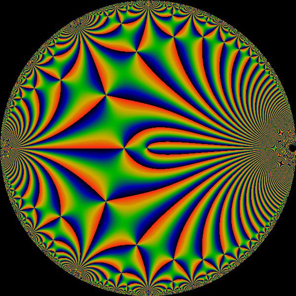
English: Klein's J-invariant, phase portrait (600x600 pixels)
Detailed descriptionThis image shows the phase of the J-invariant as a function of the square of the nome on the unit disk . That is, runs from 0 to along the edge of the disk. Black indicates regions where the phase is , green where the phase is zero, and red where the phase is . Zeros occur at the points where the colors wrap all the way around a point. Here, the tri-corner intersections show that the phase wraps around three times, for a total of , indicating that the zeros are of the third power: . The diamond-shaped patterns at the right side of the image are Moiré patterns, and are an artifact of the pixelization of the image (the strips are smaller than the size of a pixel; the color of the pixel is assigned according to the value of the function at the center of the pixel, rather than the average of values over the pixel). The fractal self-similarity of this function is that of the modular group; note that this function is a modular form. Every modular function will have this general kind of self-similarity. In this sense, this particular image clearly illustrates the tesselation of the Poincare disk by the modular group. Each quadrilateral visible in the image consists of a pair of hyperbolic triangles; each triangle is a fundamental domain of the modular group. Note in particular that one corner of each triangle lies on the edge of the disk, with exactly one exception: there is one exceptional very tiny triangle (about two pixels in size), taking the shape of an oval, that lies surrounding the center of the disk. One corner of that triangle is exactly at the center . See the image of the real part for a description of this exceptional triangle, as well as the funny exceptional tongue that goes with it. See also Image:J-inv-real.jpeg for the real part. It, and other related images, can be seen at http://www.linas.org/art-gallery/numberetic/numberetic.html Relevant Links |
| Date | 15 February 2005 (original upload date) |
| Source | Created by Linas Vepstas User:Linas <linas@linas.org> on 15 February 2005 using custom software written entirely by Linas Vepstas. |
| Author | The original uploader was Linas at English Wikipedia. |
| Permission (Reusing this file) |
Released under the Gnu Free Documentation License (GFDL) by Linas Vepstas. |


Licensing
| This file is licensed under the Creative Commons Attribution-Share Alike 3.0 Unported license. Subject to disclaimers. | ||
| ||
| This licensing tag was added to this file as part of the GFDL licensing update. |

|
Permission is granted to copy, distribute and/or modify this document under the terms of the GNU Free Documentation License, Version 1.2 or any later version published by the Free Software Foundation; with no Invariant Sections, no Front-Cover Texts, and no Back-Cover Texts. A copy of the license is included in the section entitled GNU Free Documentation License. Subject to disclaimers. |
Captioned As
| Page | Caption |
|---|---|
| Mathematics of radio engineering | A complex-valued function. |
| J-invariant | Phase of the -invariant as a function of the nome q on the unit disk |
Original upload log
| Date/Time | Dimensions | User | Comment |
|---|---|---|---|
| 2005-02-15 15:38 | 600×600× (93799 bytes) | Linas | Klein's J-invariant, phase portrait |
File history
Click on a date/time to view the file as it appeared at that time.
| Date/Time | Thumbnail | Dimensions | User | Comment | |
|---|---|---|---|---|---|
| current | 14:28, 15 December 2014 | | 600 × 600 (92 KB) | wikimediacommons>Mx. Granger | Transferred from en.wikipedia |
File usage
There are no pages that use this file.