File:Discrete probability distribution illustration.png
Jump to navigation
Jump to search
Size of this preview: 533 × 600 pixels. Other resolutions: 213 × 240 pixels | 426 × 480 pixels | 682 × 768 pixels | 910 × 1,024 pixels | 1,806 × 2,033 pixels.
Original file (1,806 × 2,033 pixels, file size: 44 KB, MIME type: image/png)
| There are SVG versions: | 
|

| |

|
Summary
| Description |
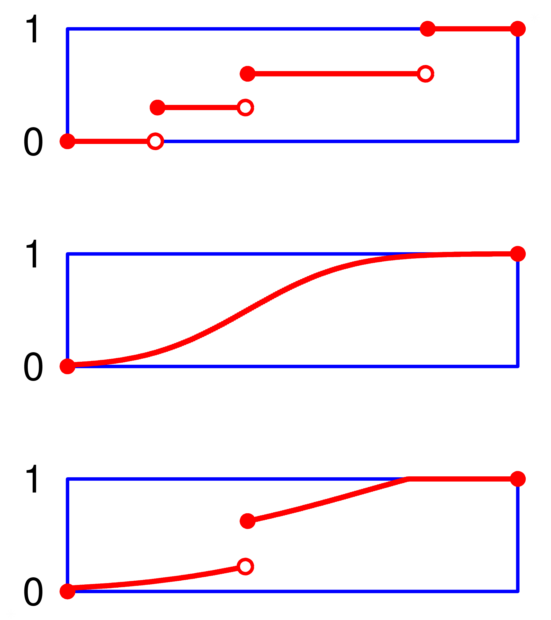
English: From top to bottom, the cumulative distribution function of a discrete probability distribution, continuous probability distribution, and a distribution which has both a continuous part and a discrete part. Cumulative distribution functions are examples of càdlàg functions.
Français : Fonctions de répartition d'une variable discrète, d'une variable diffuse et d'une variable avec atome, mais non discrète.
עברית: בשרטוט העליון מוצגת פונקציית ההצטברות של ההתפלגות הבדידה שלה שלושה ערכים אפשריים: {1}, {3} ו-{7} בהסתברות 0.2, 0.5 ו-0.3 בהתאמה. השרטוט האמצעי מציג את פונקציית ההצטברות של התפלגות רציפה, עובדה שניתן להסיק בשל רציפות הפונקציה על כל הטווח [0,1]. השרטוט התחתון מציג פונקציית הצטברות של התפלגות שהינה רציפה בחלקה ובדידה בחלקה.
Magyar: Az eloszlásfüggvények például càdlàg függvények.
Italiano: Le funzioni di ripartizione sono un esempio di funzioni càdlàg.
日本語: 上から順に、離散確率分布、連続確率分布、連続部分と離散部分がある確率分布の累積分布関数.
한국어: 이산 확률 분포, 연속 확률 분포, 이산적인 부분과 연속적인 부분이 모두 존재하는 분포에 대한 각각의 누적 분포 함수.
Polski: Od góry: dystrybuanta pewnego dyskretnego rozkładu, rozkładu ciagłego, oraz rozkładu mającego zarówno ciągłą, jak i dyskretną część.
Српски / srpski: Одозго на доле, функција расподеле дискретне случајне променљиве, непрекидне случајне променљиве, и случајне променљиве која има и непрекидне и дискретне делове.
Sunda: From top to bottom, the cumulative distribution function of a discrete probability distribution, continuous probability distribution, and a distribution which has both a continuous part and a discrete part.
Türkçe: Yukarıdan aşağıya doğru: bir ayrık olasılık dağılımı için, bir sürekli olasılık dağılımı için ve hem sürekli hem de ayrık kısımları bulunan bir olasılık dağılımı için yığmalı olasılık fonksiyonu. Üsten alta doğru. Bir aralıklı dağılım için, bir sürekli dağılım için ve hem sürekli bir kısmı hem de aralıklı bir kısmı bulunan bir dağılım için yığmalı dağılım fonksiyonları.
Українська: Зверху вниз: функція розподілу для дискретного розподілу ймовірностей, для неперервного розподілу та для розподілу що містить дискретну та неперервну частини.
Tiếng Việt: Từ trên xuống dưới, hàm phân phối tích tũy của một phân phối xác suất rời rạc, phân phối xác suất liên tục, và một phân phối có cả một phần liên tục và một phần rời rạc. Hàm phân bố tích lũy là một ví dụ của hàm số càdlàg. |
| Source | Own work |
| Author | Oleg Alexandrov |
| Other versions | see above and below |
This diagram was created with MATLAB.

|
File:Discrete probability distribution illustration.svg is a vector version of this file. It should be used in place of this PNG file.
File:Discrete probability distribution illustration.png → File:Discrete probability distribution illustration.svg
For more information, see Help:SVG. |
 |
Licensing
| I, the copyright holder of this work, release this work into the public domain. This applies worldwide. In some countries this may not be legally possible; if so: I grant anyone the right to use this work for any purpose, without any conditions, unless such conditions are required by law. |
Source code (MATLAB)
% plot a the cummulative distribution function for a
% (a) discrete distribution
% (b) continuous distribution
% (c) a distribution which has both a discrete and a continuous part

function main()

   clf; hold on; axis equal; axis off;
   L=4; h = 0.02;
   X=0:h:L;
   shift = 2;

   Y = [0*find(X < 0.2*L), 0.3+0*find( X >= 0.2*L & X < 0.4*L) 0.6+0*find(X >= 0.4*L & X < 0.8*L), 1+0*find(X>= 0.8*L)];
   plot_graph(X, Y, L, 0*shift)

   Y = 0.5*erf((4/L)*(X-L/2.5))+0.5;
   plot_graph(X, Y, L, shift);

   ds = 0.4;
   Y = 0.5*erf((2/L)*(X-L/1.5))+0.5;
   Y = Y + [0*find(X < ds*L) 0.4+0*find(X >= ds*L)]; Y = min(Y, 1);
   plot_graph(X, Y, L, 2*shift);

   % plot two dummy points to make matlab expand a bit the window before saving
   plot(L+0.15, 1.1, '*', 'color', 0.99*[1, 1, 1]);
   plot(-0.5, -2.1*shift, '*', 'color', 0.99*[1, 1, 1]);

   % save as eps
   saveas(gcf, 'Discrete_probability_distribution_illustration.eps', 'psc2')

function plot_graph(X, Y, L, shift)

   % settings
   N = length (X);
   tol = 0.1;
   thick_line = 3;
   thin_line = 2;
   small_rad = 0.07;
   red= [1, 0, 0];
   blue = [0, 0, 1];
   fs = 23;
   epsilon = 0.01;

% plot a blue box
   plot([0, L, L, 0, 0], [0, 0, 1, 1, 0]-shift, 'linewidth', thin_line, 'color', blue)

   % everything will be shifted down
   Y  = Y - shift;

   % if the given funtion has a jump, plot some balls. Otherwise plot a continous segment
   for i=1:(N-1)
      if abs(Y(i)-Y(i+1)) > tol

	 ball       (X(i+1), Y(i+1), small_rad,                red);
	 empty_ball (X(i),   Y(i),   thin_line, 0.9*small_rad, red);

      else
	 plot([X(i)-epsilon, X(i+1)+epsilon], [Y(i), Y(i+1)], 'color', red, 'linewidth', thick_line);
      end
   end

   ball       (0, -shift, small_rad,             red);
   ball       (L, 1-shift, small_rad,             red);

%plot text
   small= 0.4;
   text(-small, 0-shift, '0', 'fontsize', fs)
   text(-small, 1-shift, '1', 'fontsize', fs)


function ball(x, y, r, color)
   Theta=0:0.1:2*pi;
   X=r*cos(Theta)+x;
   Y=r*sin(Theta)+y;
   H=fill(X, Y, color);
   set(H, 'EdgeColor', 'none');


function empty_ball(x, y, thick_line, r, color)
   Theta=0:0.1:2*pi;
   X=r*cos(Theta)+x;
   Y=r*sin(Theta)+y;
   H=fill(X, Y, [1 1 1]);
   plot(X, Y, 'color', color, 'linewidth', thick_line);
File history
Click on a date/time to view the file as it appeared at that time.
| Date/Time | Thumbnail | Dimensions | User | Comment | |
|---|---|---|---|---|---|
| current | 17:51, 12 May 2007 | | 1,806 × 2,033 (44 KB) | wikimediacommons>Oleg Alexandrov | {{Information |Description= |Source=self-made |Date= |Author= User:Oleg Alexandrov }} Made with matlab. {{PD-self}} |
File usage
There are no pages that use this file.