File:Discontinuity jump.eps.png
Jump to navigation
Jump to search
Size of this preview: 643 × 599 pixels. Other resolutions: 258 × 240 pixels | 515 × 480 pixels | 824 × 768 pixels | 1,099 × 1,024 pixels | 2,122 × 1,978 pixels.
Original file (2,122 × 1,978 pixels, file size: 81 KB, MIME type: image/png)
Transferred from en.wikipedia to Commons by Maksim.
The original description page was here. All following user names refer to en.wikipedia.
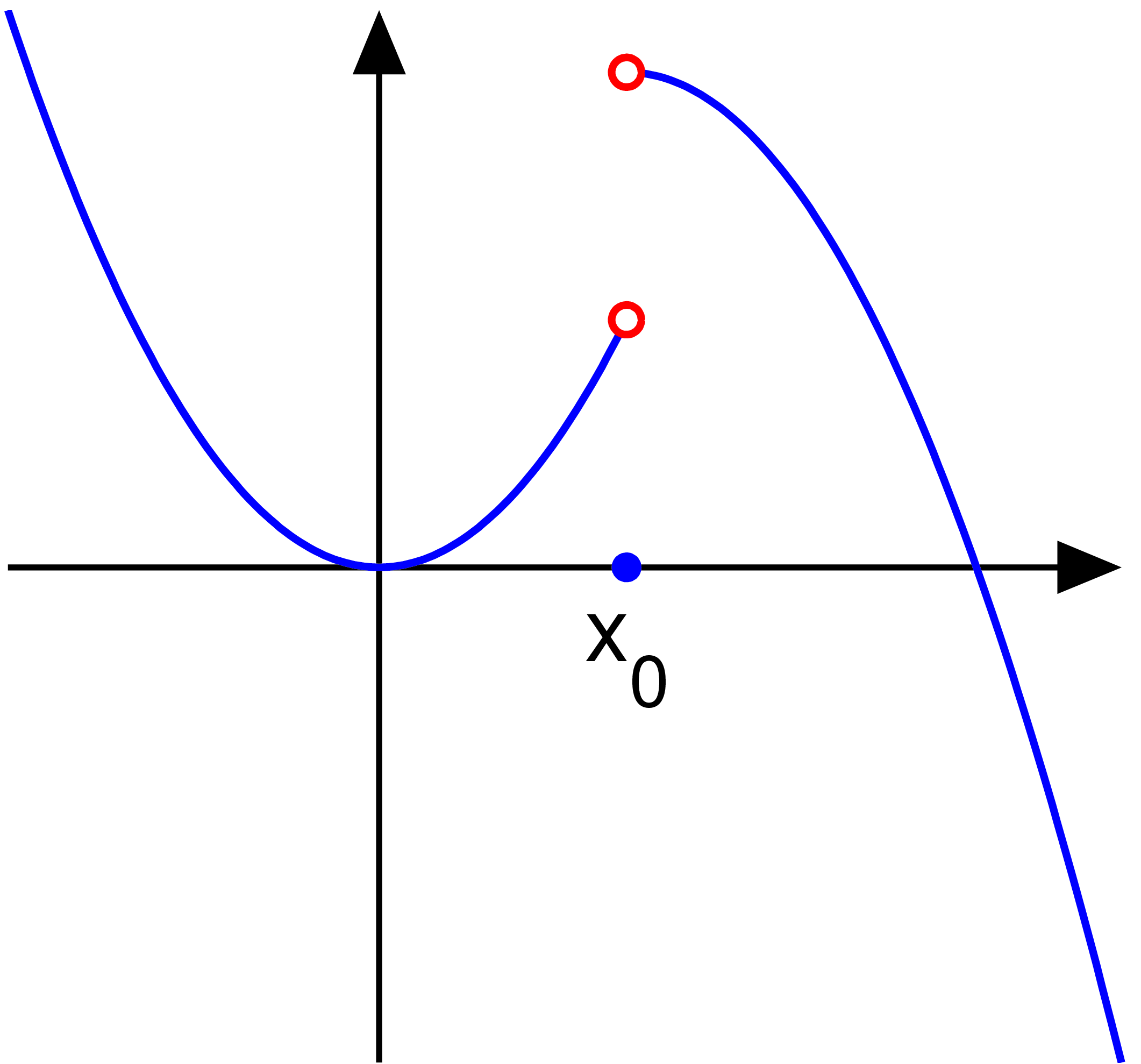
Summary
Made by me with matlab. {PD.}
This diagram was created with MATLAB.
Licensing
| I, the copyright holder of this work, release this work into the public domain. This applies worldwide. In some countries this may not be legally possible; if so: I grant anyone the right to use this work for any purpose, without any conditions, unless such conditions are required by law. |
Source code (MATLAB)
function discontinuity()

   % set up the plotting window
   thick_line=2.5; thin_line=2; arrow_size=14; arrow_type=2;
   fs=30; circrad=0.06;

% picture 1
   a=-1.5; b=3; h=0.02; x0=1;
   X1=a:h:x0; X2=x0:h:b; X=[X1 X2];
   Y1=X1.^2; Y2=Y1(length(Y1))+(-1)*(X2-X2(1)); Y=[Y1 Y2]; y01=Y1(length(Y1)); y02=Y2(1);

   figure(1); clf; hold on; axis equal; axis off;
   axes_points(a, b, thin_line, thick_line, arrow_size, arrow_type, x0, y01, y02, circrad, fs, X, Y, X1, Y1, X2, Y2)
   saveas(gcf, 'discontinuity_removable.eps', 'psc2')

% picture 2
   a=-1.5; b=3; h=0.02; x0=1;
   X1=a:h:x0; X2=x0:h:b; X=[X1 X2];
   Y1=X1.^2; Y2=2-(X2-x0).^2; Y=[Y1 Y2]; y01=Y1(length(Y1)); y02=Y2(1);

   figure(2); clf; hold on; axis equal; axis off;
   axes_points(a, b, thin_line, thick_line, arrow_size, arrow_type, x0, y01, y02, circrad, fs, X, Y, X1, Y1, X2, Y2)
   saveas(gcf, 'discontinuity_jump.eps', 'psc2')

% picture 3
   a=-1.5; b=3; h=0.001; x0=1;
   X1=a:h:x0; X2=x0:h:b; X=[X1 X2];
   Y1=sin(5./(X1-x0-eps)); Y2=0.1./(X2-x0+50*h); Y=[Y1 Y2]; y01=Y1(length(Y1)); y02=Y2(1);

   figure(3); clf; hold on; axis equal; axis off;
   axes_points2(a, b, thin_line, thick_line, arrow_size, arrow_type, x0, NaN, NaN, circrad, fs, X, Y, X1, Y1, X2, Y2)
   saveas(gcf, 'discontinuity_essential.eps', 'psc2')

disp('Converting to png...')
! convert -density 400 -antialias discontinuity_removable.eps discontinuity_removable.png
! convert -density 400 -antialias discontinuity_jump.eps discontinuity_jump.png
! convert -density 400 -antialias discontinuity_essential.eps discontinuity_essential.png

function axes_points(a, b, thin_line, thick_line, arrow_size, arrow_type, x0, y01, y02, circrad, fs, X, Y, X1, Y1, X2, Y2)
   arrow([a 0], [b, 0], thin_line, arrow_size, pi/8,arrow_type, [0, 0, 0]) % xaxis
   small=0.2; arrow([0, min(Y)], [0, max(Y)], thin_line, arrow_size, pi/8,arrow_type, [0, 0, 0]); % y axis

   plot(X1, Y1, 'linewidth', thick_line); plot(X2, Y2, 'linewidth', thick_line)

   ball(x0, 0, circrad, [0 0 1 ]);
   ball_empty(x0, y01, thick_line, circrad, [1 0 0 ]); ball_empty(x0, y02, thick_line, circrad, [1 0 0 ]);
   H=text(x0, -0.006*fs,  'x_0'); set(H, 'fontsize', fs, 'HorizontalAlignment', 'c', 'VerticalAlignment', 'c')

function axes_points2(a, b, thin_line, thick_line, arrow_size, arrow_type, x0, y01, y02, circrad, fs, X, Y, X1, Y1, X2, Y2)
   arrow([a 0], [b, 0], thin_line, arrow_size, pi/8,arrow_type, [0, 0, 0]) % xaxis
   small=0.2; arrow([0, min(Y)], [0, max(Y)], thin_line, arrow_size, pi/8,arrow_type, [0, 0, 0]); % y axis

   plot(X1, Y1, 'linewidth', thick_line); plot(X2, Y2, 'linewidth', thick_line)

   ball(x0, 0, circrad, [0 0 1 ]);
   ball_empty(x0, y01, thick_line, circrad, [1 0 0 ]); ball_empty(x0, y02, thick_line, circrad, [1 0 0 ]);
   H=text(x0+0.2, -0.006*fs,  'x_0'); set(H, 'fontsize', fs, 'HorizontalAlignment', 'c', 'VerticalAlignment', 'c')

function ball(x, y, r, color)
   Theta=0:0.1:2*pi;
   X=r*cos(Theta)+x;
   Y=r*sin(Theta)+y;
   H=fill(X, Y, color);
   set(H, 'EdgeColor', 'none');

function ball_empty(x, y, thick_line, r, color)
   Theta=0:0.1:2*pi;
   X=r*cos(Theta)+x;
   Y=r*sin(Theta)+y;
   H=fill(X, Y, [1 1 1]);
   %set(H, 'EdgeColor', color);
  plot(X, Y, 'color', color, 'linewidth', thick_line);

function arrow(start, stop, thickness, arrowsize, sharpness, arrow_type, color)

%  draw a line with an arrow at the end
%  start is the x,y point where the line starts
%  stop is the x,y point where the line stops
%  thickness is an optional parameter giving the thickness of the lines
%  arrowsize is an optional argument that will give the size of the arrow
%  It is assumed that the axis limits are already set
%  0 < sharpness < pi/4 determines how sharp to make the arrow
%  arrow_type draws the arrow in different styles. Values are 0, 1, 2, 3.

%       8/4/93    Jeffery Faneuff
%       Copyright (c) 1988-93 by the MathWorks, Inc.
%       Modified by Oleg Alexandrov 2/16/03

   if nargin <=6
      color=[0, 0, 0];
   end

   if (nargin <=5)
      arrow_type=0;   % the default arrow, it looks like this: ->
   end

   if (nargin <=4)
      sharpness=pi/4; % the arrow sharpness - default = pi/4
   end

   if nargin<=3
      xl = get(gca,'xlim');
      yl = get(gca,'ylim');
      xd = xl(2)-xl(1);
      yd = yl(2)-yl(1);
      arrowsize = (xd + yd) / 2;   % this sets the default arrow size
   end

   if (nargin<=2)
      thickness=0.5; % default thickness
   end

   xdif = stop(1) - start(1);
   ydif = stop(2) - start(2);

   if (xdif == 0)
      if (ydif >0)
         theta=pi/2;
      else
         theta=-pi/2;
      end
   else
      theta = atan(ydif/xdif);  % the angle has to point according to the slope
   end

   if(xdif>=0)
      arrowsize = -arrowsize;
   end

   if (arrow_type == 0) % draw the arrow like two sticks originating from its vertex
      xx = [start(1), stop(1),(stop(1)+0.02*arrowsize*cos(theta+sharpness)),NaN,stop(1),...
            (stop(1)+0.02*arrowsize*cos(theta-sharpness))];
      yy = [start(2), stop(2), (stop(2)+0.02*arrowsize*sin(theta+sharpness)),NaN,stop(2),...
            (stop(2)+0.02*arrowsize*sin(theta-sharpness))];
      plot(xx,yy, 'LineWidth', thickness, 'color', color)
   end

   if (arrow_type == 1)  % draw the arrow like an empty triangle
      xx = [stop(1),(stop(1)+0.02*arrowsize*cos(theta+sharpness)), ...
            stop(1)+0.02*arrowsize*cos(theta-sharpness)];
      xx=[xx xx(1) xx(2)];

      yy = [stop(2),(stop(2)+0.02*arrowsize*sin(theta+sharpness)), ...
            stop(2)+0.02*arrowsize*sin(theta-sharpness)];
      yy=[yy yy(1) yy(2)];

      plot(xx,yy, 'LineWidth', thickness, 'color', color)

%     plot the arrow stick
      plot([start(1) stop(1)+0.02*arrowsize*cos(theta)*cos(sharpness)], [start(2), stop(2)+ ...
                    0.02*arrowsize*sin(theta)*cos(sharpness)], 'LineWidth', thickness, 'color', color)

   end

   if (arrow_type==2) % draw the arrow like a full triangle
      xx = [stop(1),(stop(1)+0.02*arrowsize*cos(theta+sharpness)), ...
            stop(1)+0.02*arrowsize*cos(theta-sharpness),stop(1)];

      yy = [stop(2),(stop(2)+0.02*arrowsize*sin(theta+sharpness)), ...
            stop(2)+0.02*arrowsize*sin(theta-sharpness),stop(2)];
      H=fill(xx, yy, color);% fill with black
      set(H, 'EdgeColor', 'none')

%     plot the arrow stick
      plot([start(1) stop(1)+0.01*arrowsize*cos(theta)], [start(2), stop(2)+ ...
                    0.01*arrowsize*sin(theta)], 'LineWidth', thickness, 'color', color)
   end

   if (arrow_type==3) % draw the arrow like a filled 'curvilinear' triangle
      curvature=0.5; % change here to make the curved part more curved (or less curved)
      radius=0.02*arrowsize*max(curvature, tan(sharpness));
      x1=stop(1)+0.02*arrowsize*cos(theta+sharpness);
      y1=stop(2)+0.02*arrowsize*sin(theta+sharpness);
      x2=stop(1)+0.02*arrowsize*cos(theta)*cos(sharpness);
      y2=stop(2)+0.02*arrowsize*sin(theta)*cos(sharpness);
      d1=sqrt((x1-x2)^2+(y1-y2)^2);
      d2=sqrt(radius^2-d1^2);
      d3=sqrt((stop(1)-x2)^2+(stop(2)-y2)^2);
      center(1)=stop(1)+(d2+d3)*cos(theta);
      center(2)=stop(2)+(d2+d3)*sin(theta);

      alpha=atan(d1/d2);
      Alpha=-alpha:0.05:alpha;
      xx=center(1)-radius*cos(Alpha+theta);
      yy=center(2)-radius*sin(Alpha+theta);
      xx=[xx stop(1) xx(1)];
      yy=[yy stop(2) yy(1)];

      H=fill(xx, yy, color);% fill with black
      set(H, 'EdgeColor', 'none')

%     plot the arrow stick
      plot([start(1) center(1)-radius*cos(theta)], [start(2), center(2)- ...
                    radius*sin(theta)], 'LineWidth', thickness, 'color', color);
   end
| date/time | username | edit summary |
|---|---|---|
| 04:49, 5 December 2005 | en:User:Oleg Alexandrov | (clean up code) |
| 00:01, 22 November 2005 | en:User:Oleg Alexandrov | (+ source code) |
| 00:52, 12 September 2005 | en:User:Oleg Alexandrov | (Made by me with matlab. {PD.}) |
Original upload log
Legend: (cur) = this is the current file, (del) = delete this old version, (rev) = revert to this old version.
Click on date to download the file or see the image uploaded on that date.
- (del) (cur) 10:30, 20 January 2006 . . DavidHouse ( en:User_talk:DavidHouse Talk) . . 318x297 (10408 bytes) (Reverted to earlier revision)
- (del) (rev) 10:30, 20 January 2006 . . DavidHouse ( en:User_talk:DavidHouse Talk) . . 317x297 (8531 bytes) (Reverted to earlier revision)
- (del) (rev) 01:28, 12 September 2005 . . en:User:Oleg_Alexandrov Oleg Alexandrov ( en:User_talk:Oleg_Alexandrov Talk) . . 318x297 (10408 bytes)
- (del) (rev) 00:52, 12 September 2005 . . en:User:Oleg_Alexandrov Oleg Alexandrov ( en:User_talk:Oleg_Alexandrov Talk) . . 317x297 (8531 bytes) (Made by me with matlab. { PD. })
derivative works
Derivative works of this file: Not defined at x0.svg

|
This math image could be re-created using vector graphics as an SVG file. This has several advantages; see Commons:Media for cleanup for more information. If an SVG form of this image is available, please upload it and afterwards replace this template with
{{vector version available|new image name}}.
It is recommended to name the SVG file “Discontinuity jump.eps.svg”—then the template Vector version available (or Vva) does not need the new image name parameter. |
File history
Click on a date/time to view the file as it appeared at that time.
| Date/Time | Thumbnail | Dimensions | User | Comment | |
|---|---|---|---|---|---|
| current | 06:17, 11 July 2013 | | 2,122 × 1,978 (81 KB) | wikimediacommons>Oleg Alexandrov | Made the point on the axis blue, per request, this is how it should be. |
File usage
There are no pages that use this file.