Main Page: Difference between revisions
No edit summary |
No edit summary |
||
| Line 1: | Line 1: | ||
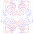
[[File:Slope Field.png|thumb|right|250px|The slope field of dy/dx=x<sup>2</sup>-x-2, with the blue, red, and turquoise lines being (x<sup>3</sup>/3)-(x<sup>2</sup>/2)-2x+4, (x<sup>3</sup>/3)-(x<sup>2</sup>/2)-2x, and (x<sup>3</sup>/3)-(x<sup>2</sup>/2)-2x-4, respectively.]] | |||
In [[mathematics]], a '''slope field''' (or '''direction field''') is a graphical representation of the solutions of a first-order [[differential equation]]. It is useful because it can be created without solving the differential equation analytically. The representation may be used to qualitatively visualize solutions, or to numerically approximate them. | |||
==Definition== | |||
===Standard case=== | |||
The slope field is traditionally defined for the following type of differential equations | |||
:<math>y'=f(x,y)</math>. | |||
It can be viewed as a creative way to plot a real-valued function of two real variables <math>f(x,y)</math> as a planar picture. Specifically, for a given pair <math>x,y</math>, a vector with the components <math>[1, f(x,y)]</math> is drawn at the point <math>x,y</math> on the <math>x,y</math>-plane. Sometimes, the vector <math>[1, f(x,y)]</math> is normalized to make the plot better looking for a human eye. A set of pairs <math>x,y</math> making a rectangular grid is typically used for the drawing. | |||
An [[Isocline]] (a series of lines with the same slope) is often used to supplement the slope field. In an equation of the form <math>y'=f(x,y)</math>, the isocline is a line in the <math>x,y</math>-plane plane obtained by setting <math>f(x,y)</math> equal to a constant. | |||
===General case of a system of differential equations=== | |||
Given a system of differential equations, | |||
:<math>\frac{dx_1}{dt}=f_1(t,x_1,x_2,\ldots,x_n)</math> | |||
:<math>\frac{dx_2}{dt}=f_2(t,x_1,x_2,\ldots,x_n)</math> | |||
:::<math>\vdots</math> | |||
:<math>\frac{dx_n}{dt}=f_n(t,x_1,x_2,\ldots,x_n)</math> | |||
the slope field is an array of slope marks in the [[phase space]] (in any number of dimensions depending on the number of relevant variables; for example, two in the case of a first-order linear [[ordinary differential equation|ODE]], as seen to the right). Each slope mark is centered at a point <math>(t,x_1,x_2,\ldots,x_n)</math> and is parallel to the vector | |||
The | :<math>\begin{pmatrix} 1 \\ f_1(t,x_1,x_2,\ldots,x_n) \\ f_2(t,x_1,x_2,\ldots,x_n) \\ \vdots \\ f_n(t,x_1,x_2,\ldots,x_n) \end{pmatrix}</math>. | ||
The number, position, and length of the slope marks can be arbitrary. The positions are usually chosen such that the points <math>(t,x_1,x_2,\ldots,x_n)</math> make a uniform grid. The standard case, described above, represents <math>n=1</math>. The general case of the slope field for systems of differential equations is not easy to visualize for <math>n>2</math>. | |||
==General application== | |||
With computers, complicated slope fields can be quickly made without tedium, and so an only recently practical application is to use them merely to get the feel for what a solution should be before an explicit general solution is sought. Of course, computers can also just solve for one, if it exists. | |||
If there is no explicit general solution, computers can use slope fields (even if they aren’t shown) to numerically find graphical solutions. Examples of such routines are [[Euler's method]], or better, the [[Runge-Kutta methods]]. | |||
== | ==Software for plotting slope fields== | ||
Different software packages can plot slope fields. | |||
===Example code in [[GNU Octave]]/[[MATLAB]] === | |||
<source lang="matlab"> | |||
Ffun = @(X,Y)X.*Y; % function f(x,y)=xy | |||
[X,Y]=meshgrid(-2:.3:2,-2:.3:2); % choose the plot sizes | |||
DY=Ffun(X,Y); DX=ones(size(DY)); % generate the plot values | |||
quiver(X,Y,DX,DY); % plot the direction field | |||
hold on; | |||
contour(X,Y,DY,[-6 -2 -1 0 1 2 6]); %add the isoclines | |||
title('Slope field and isoclines for f(x,y)=xy') | |||
</source> | |||
===Alternate example code in [[GNU Octave]]/[[MATLAB]] === | |||
<source lang="matlab"> | |||
funn = @(x,y)y-x; % function f(x,y)=y-x | |||
[x,y]=meshgrid(-2:0.5:2); % intervals for x and y | |||
slopes=funn(x,y); % matrix of slopes | |||
dy=slopes./sqrt(1+slopes.^2); % normalize the line element... | |||
dx=sqrt(1-dy.^2); % ...magnitudes for dy and dx | |||
quiver(x,y,dx,dy); % plot the direction field | |||
</source> | |||
=== Example code for [[Maxima (software) | Maxima]] === | |||
/* field for y'=xy (click on a point to get an integral curve) */ | |||
plotdf( x*y, [x,-2,2], [y,-2,2]); | |||
==Examples== | |||
<gallery Caption="y' = xy"> | |||
Image:Slope_field_1.svg|Slope field | |||
Image:Slope_field_with_integral_curves_1.svg|Integral curves | |||
image:Isocline_3.png|Isoclines (blue), slope field (black), and some solution curves (red) | |||
</gallery> | |||
== | |||
: | |||
: | |||
and | |||
==See also== | ==See also== | ||
* [[ | *[[Examples of differential equations]] | ||
* [[ | *[[Vector field]] | ||
*[[Laplace transform applied to differential equations]] | |||
*[[List of dynamical systems and differential equations topics]] | |||
==References== | ==References== | ||
* | * Blanchard, Paul; Devaney, Robert L.; and Hall, Glen R. (2002). ''Differential Equations'' (2nd ed.). Brooks/Cole: Thompson Learning. ISBN 0-534-38514-1 | ||
==External links== | |||
* {{MathWorld |title = Slope field |urlname = SlopeField}} | |||
* [http://www.math.psu.edu/cao/DFD/Dir.html Slope field plotter] | |||
[[Category: | [[Category:Calculus]] | ||
[[Category: | [[Category:Differential equations]] | ||
[[Category: | [[Category:Articles with example MATLAB/Octave code]] | ||
Revision as of 03:32, 14 August 2014

In mathematics, a slope field (or direction field) is a graphical representation of the solutions of a first-order differential equation. It is useful because it can be created without solving the differential equation analytically. The representation may be used to qualitatively visualize solutions, or to numerically approximate them.
Definition
Standard case
The slope field is traditionally defined for the following type of differential equations
- .

It can be viewed as a creative way to plot a real-valued function of two real variables as a planar picture. Specifically, for a given pair , a vector with the components is drawn at the point on the -plane. Sometimes, the vector is normalized to make the plot better looking for a human eye. A set of pairs making a rectangular grid is typically used for the drawing.


![{\displaystyle [1,f(x,y)]}](https://wikimedia.org/api/rest_v1/media/math/render/svg/47b0f1a2b509928c2c7981d32549930250732a24)
An Isocline (a series of lines with the same slope) is often used to supplement the slope field. In an equation of the form , the isocline is a line in the -plane plane obtained by setting equal to a constant.
General case of a system of differential equations
Given a system of differential equations,


the slope field is an array of slope marks in the phase space (in any number of dimensions depending on the number of relevant variables; for example, two in the case of a first-order linear ODE, as seen to the right). Each slope mark is centered at a point and is parallel to the vector

- .

The number, position, and length of the slope marks can be arbitrary. The positions are usually chosen such that the points make a uniform grid. The standard case, described above, represents . The general case of the slope field for systems of differential equations is not easy to visualize for .


General application
With computers, complicated slope fields can be quickly made without tedium, and so an only recently practical application is to use them merely to get the feel for what a solution should be before an explicit general solution is sought. Of course, computers can also just solve for one, if it exists.
If there is no explicit general solution, computers can use slope fields (even if they aren’t shown) to numerically find graphical solutions. Examples of such routines are Euler's method, or better, the Runge-Kutta methods.
Software for plotting slope fields
Different software packages can plot slope fields.
Example code in GNU Octave/MATLAB
Ffun = @(X,Y)X.*Y;               % function f(x,y)=xy
[X,Y]=meshgrid(-2:.3:2,-2:.3:2); % choose the plot sizes
DY=Ffun(X,Y); DX=ones(size(DY)); % generate the plot values
quiver(X,Y,DX,DY);               % plot the direction field
hold on;
contour(X,Y,DY,[-6 -2 -1 0 1 2 6]); %add the isoclines
title('Slope field and isoclines for f(x,y)=xy')
Alternate example code in GNU Octave/MATLAB
funn = @(x,y)y-x;                % function f(x,y)=y-x
[x,y]=meshgrid(-2:0.5:2);        % intervals for x and y
slopes=funn(x,y);                % matrix of slopes
dy=slopes./sqrt(1+slopes.^2);    % normalize the line element...
dx=sqrt(1-dy.^2);                % ...magnitudes for dy and dx
quiver(x,y,dx,dy);               % plot the direction field
Example code for Maxima
/* field for y'=xy (click on a point to get an integral curve) */
plotdf( x*y, [x,-2,2], [y,-2,2]);
Examples
- y' = xy
-
Slope field
-
Integral curves
-
Isoclines (blue), slope field (black), and some solution curves (red)

See also
- Examples of differential equations
- Vector field
- Laplace transform applied to differential equations
- List of dynamical systems and differential equations topics
References
- Blanchard, Paul; Devaney, Robert L.; and Hall, Glen R. (2002). Differential Equations (2nd ed.). Brooks/Cole: Thompson Learning. ISBN 0-534-38514-1
External links
I had like 17 domains hosted on single account, and never had any special troubles. If you are not happy with the service you will get your money back with in 45 days, that's guaranteed. But the Search Engine utility inside the Hostgator account furnished an instant score for my launched website. Fantastico is unable to install WordPress in a directory which already have any file i.e to install WordPress using Fantastico the destination directory must be empty and it should not have any previous installation files. When you share great information, others will take note. Once your hosting is purchased, you will need to setup your domain name to point to your hosting. Money Back: All accounts of Hostgator come with a 45 day money back guarantee. If you have any queries relating to where by and how to use Hostgator Discount Coupon, you can make contact with us at our site. If you are starting up a website or don't have too much website traffic coming your way, a shared plan is more than enough. Condition you want to take advantage of the worldwide web you prerequisite a HostGator web page, -1 of the most trusted and unfailing web suppliers on the world wide web today. Since, single server is shared by 700 to 800 websites, you cannot expect much speed.
Hostgator tutorials on how to install Wordpress need not be complicated, especially when you will be dealing with a web hosting service that is friendly for novice webmasters and a blogging platform that is as intuitive as riding a bike. After that you can get Hostgator to host your domain and use the wordpress to do the blogging. Once you start site flipping, trust me you will not be able to stop. I cut my webmaster teeth on Control Panel many years ago, but since had left for other hosting companies with more commercial (cough, cough) interfaces. If you don't like it, you can chalk it up to experience and go on. First, find a good starter template design. When I signed up, I did a search for current "HostGator codes" on the web, which enabled me to receive a one-word entry for a discount. Your posts, comments, and pictures will all be imported into your new WordPress blog.- Slope field plotter